How To Create A Company Budget In Excel?
1. Click on the Excel icon in your computer and start up a new blank spreadsheet.
2. Click on the first row and type the name of the excel spreadsheet. Click the second cell on the third row and type the first expenditure for the business. Move to the next row and type another expense. Continue in that manner until you have typed in all the expenses for the business such as Travel, Utilities, Office Rent, Insurance, etc.
3. Go to the first column and put the cursor on the fourth cell (this would be A4). Add the name of the department for which the budget is prepared or the name of employees who have spending/purchasing powers within the organization. Click the ENTER key to move to the next cell. Enter the next name and press ENTER. Continue this process until all sections involved in the company’s budget are entered.
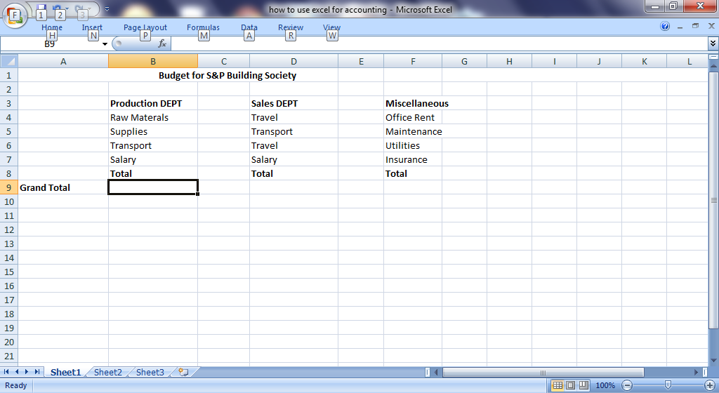
4. Click and highlight all entries in the first column. Right click and then click the “format Cell” option to color-fill each of the cells with different colors to make them stand out from each other. Go over to the font tab and change the font style to “bold”. After this is done, you need to click the OK bottom for excel to automatically affect the changes.
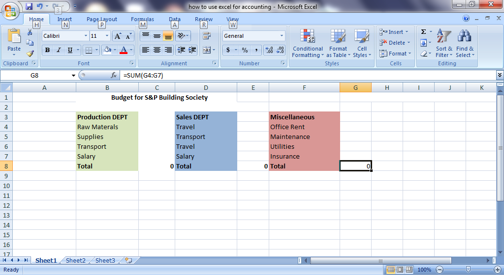
5. Go over to the expense section in row three to carry out the same formatting. Click and highlight the worksheet’s title and carry out the same formatting, but this time make the words larger than the headings so that they are slightly different from the heading. Use the AUTOSUM feature of the spreadsheet to make your calculations simpler. Highlight the cells in one column (such as the cells under office rent) and click the “autosum” button. The cells will fill up with the symbol =SUM (). This tells you that the cells will add up automatically when they are imputed into the spreadsheet, providing a monthly sum for the column.
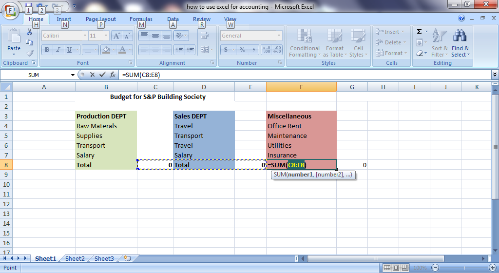
6. The next step is to highlight the new AUTOSUM cell in the spreadsheet row as well as one blank cell. Then use the AUTOSUM feature to add up the monthly budget. This total will show up in the new blank cell.

7. After all entries have been made and the autosum feature is running, open the file tab and select “SAVE AS”, type the name of the spreadsheet and save to the computer. Your accounting spreadsheet in your excel is up and running.
Bottom line
Once the Excel spreadsheet is up and running, any monthly addition to the budget will be updated automatically because of the autosum feature. All you need to do is type in the expense amount under the proper name at the expense column. Excel will automatically sum up the figure and update the data from previous month’s expenses. The original worksheet you will create by following the above steps will remain the template each time you want to make an update on the budget.
At the end, your Excel spreadsheet should look like this:
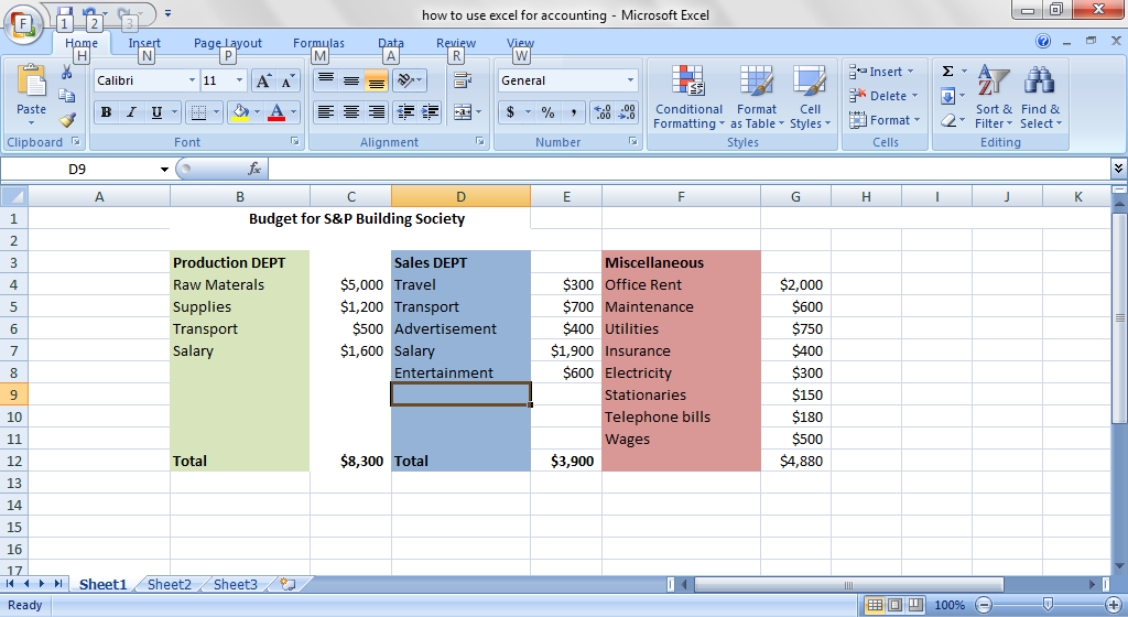
You can leave some spaces (as shown in the screenshot above) where you can enter more expenses as they are incurred. Once you enter the name and amount of expense, hit the enter button and the total amount will be updated automatically.
Template
Further reading:
Basic concepts
Getting started with Excel
Cell References


