

Data Validation in Excel
MS Excel is the most popular spreadsheet software with a wide range of features, formulas, and functions. Data Validation is one of the essential features in MS Excel. When creating an Excel sheet for users or customers, we may often need to restrict the inputs based on different criteria to ensure that all the entries or inputs are correct and consistent. Data Validation is the solution that helps us control user inputs into specific cells or a range according to the specified rules.
In this article, we discuss the feature Data Validation in Excel and the method to insert/ apply it within the Excel sheet. The article also explains relevant examples with images to help us understand the concepts of Data Validation clearly.
What is Data Validation?
Data Validation is an essential Excel feature that helps control or restrict user inputs/ entries in selected cells. It enables users to set the desired validation rules to control what type of data they can enter into the corresponding cells in an Excel sheet. For instance, we can restrict users to enter values between 1 to 10, enter names or passwords in less than 30 characters, enter or choose an entry from the predefined list of acceptable values, and more.
Some of the essential tasks (restrictions/ validations) that we can set using the Data Validation are as follows:
- Allow users to put numeric or text entries only
- Allow entering numbers less than, more than and between a specified range
- Allow data inputs of a specific length
- Restrict entries to predefined values in a drop-down list
- Restrict date and time entries outside or within a specific range
- Validate a specific entry based on another cell
- Display an input message informing users what the corresponding cell accepts when the user selects a cell
- Display a warning or error message when the user enters wrong data
- Locate incorrect or wrong entries in the validated cells
Note: It should be noted that the data validation feature is not a completely reliable way to control input and can be easily defeated. If we copy data from cells with no validation rules and then paste those cells to cells with data validation, the validation is destroyed. Specifically, validation rules are removed or changed from the corresponding cell based on the copied cells.
How does Data Validation work in Excel?
Applying Data Validation on any cell or range of cells in an Excel sheet restricts the users from entering any undesired entries in corresponding cells based on the validation rules. For instance, if we set validation to accept only numbers or numeric values, other users or we will not be able to enter any values other than numbers.
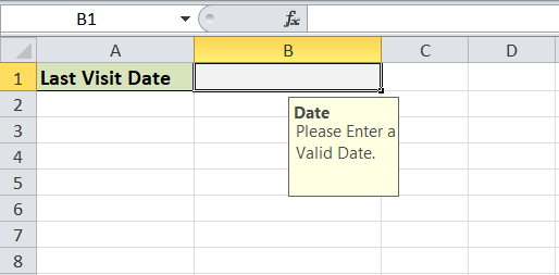
Data Validation can be configured to show an input message to users when the respective cell is selected, informing them what is allowed in it, as shown below:
As soon as we try to enter any other type of data in restricted cells, Excel instantly displays an error message and even can display which type of data the respective cells can accept. The error message can be of different styles and customized or created manually while setting up the validation rules on the Excel sheet.
Data Validation Controls
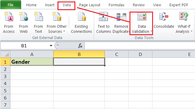
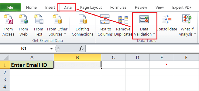
The Data Validation feature or its controls can be found on the ribbon under the Data tab. By default, it is placed under the category ‘Data Tools’.
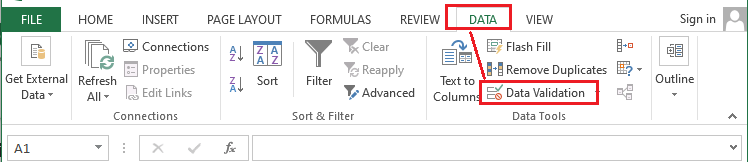
As soon we click the ‘Data Validation’ icon from the ribbon, it immediately launched a Data Validation dialogue box.
In addition to the Data Validation shortcut on the ribbon, we can also use the keyboard shortcut ‘Alt + D + L‘ without quotes. It will launch the Data Validation dialogue box instantly.
Using Data Validation Dialog Box to Define Validation Rules
The Data Validation dialogue box contains three essential options/ tabs: Settings, Input Message, and Error Alert.
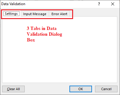
Let us understand each tab in detail:
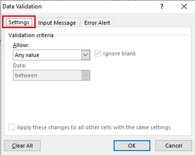
Settings Tab
The settings tab provides us options to set validation criteria. The tab helps us choose the desired validation rules from the built-in options we want to allow in selected cells. Moreover, we can also set custom rules with the customized formula to validate user inputs. The settings tab contains all the data validation options present in Excel.
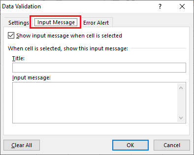
Input Message Tab
The input message tab has a text box to enter a message displayed as soon as the respective cell is selected. The input message is an optional feature of Data Validation. If we do not define any message as an input message, excel does not show any message when the user selects the respective cell with data validation. It does not affect the working of the data validation and has no effect or control over what the user enters into a cell. However, it can be helpful to inform users about the allowed or expected data values.
Error Alert Tab
The error alert tab provides us options to control the way how the validation is enforced. We can set criteria and then use any desired error style to accept or reject the user inputs accordingly. Additionally, we can also display a message to the user informing what the error is or what values must be entered in corresponding cells.
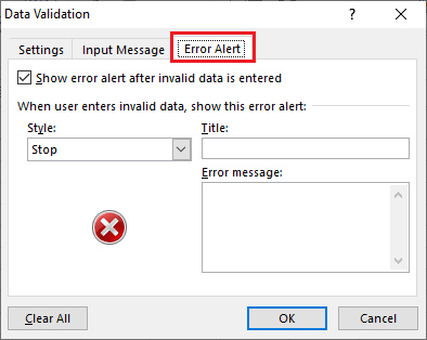
There are currently three types of error styles in MS Excel, as listed below:
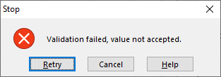
- Stop: When the error style is set to ‘Stop’, Excel prevents users from entering invalid data in respective cells. If a user enters invalid data, it triggers a pop-up window with a specified message, and the input is rejected. The Stop alert window displays two options: Retry (to edit invalid data) and Cancel (to remove the invalid data). Although the Stop Alert window displays options to retry, users must enter the correct value, which passes validation when retrying.

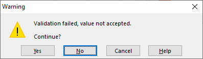
- Warning: When the error style is set to ‘Warning’, Excel warns users that the entered value is invalid. It also displays a different icon and the specified message. However, it does not prevent users from entering invalid values; users can ignore the warning message and register a value that does not even pass the validation. The Warning alert window displays three options: Yes (to accept invalid data), No (to edit invalid data) and Cancel (to remove the invalid data).
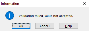
- Information: When the error style is set to ‘Information’, Excel informs users that the entered data is invalid. It displays a different icon and a specified message. Like the Warning error style, the Information error style also does nothing to prevent invalid data. Users can ignore the information message and register invalid data without passing the validation. The Information alert window displays two options: OK (to accept invalid data) and Cancel (to remove the invalid data).
Data Validation Options
When creating a data validation rule from the settings tab, we have eight options to validate user inputs. They are as follows:
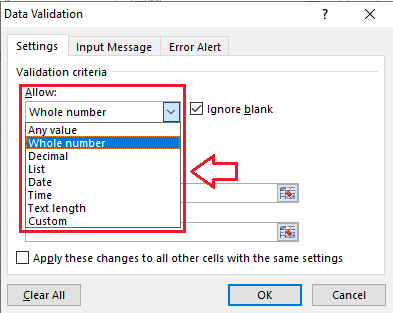
- Any Value: It removes restrictions and allows every value in selected cells, making no validation at all. However, data validation in selected cells earlier with an input message displays the message while selecting the respective cells. Therefore, we must edit/ remove the input message when selecting the option ‘Any Value’.
- Whole Number: It restricts users to enter only the whole numbers. Once we select the’ Whole Number’ option, we get more options relevant to limiting user inputs. The other options typically include less than, more than, equal to, between, etc. For instance, we can restrict users to enter whole numbers between 1 to 100 in restricted cells.
- Decimal: It is almost identical to the option ‘Whole Number’. However, it allows users to enter values in decimal forms. For instance, if we restrict users to enter decimal values between 0 to 5, the respective cells can accept values like 2.3, 0.5, 0.9, 4.1, etc.
- List: It is a typical type of validation. It restricts users to select values from a predefined list. Specifically, the predefined values are displayed to the user in the form of a drop-down menu. We can define values directly into the Settings tab or supply them as a range on the sheet. For instance, we can restrict users to select a Gender from a list having values like Male, Female and Others.
- Date: It restricts users to enter values in the dates form. However, we can set some validation rules to allow previous dates, futures dates, dates between the specific range, etc. For instance, we can restrict cells to accept only the future dates in the appointment row/column.
- Time: It is almost identical to the option ‘Date’. However, it restricts users to enter times. We can set validations to allow time before, after a specific time, or between specific time ranges. For instance, we can restrict cells to accept time between 8:00 AM and 7:00 PM.
- Text Length: It restricts users to enter values of the specific length. This typically means that the inputs are validated according to the number of characters or digits. For instance, if we restrict users to enter values with length 4 in the desired cells, the specified cells can only accept values with four characters or digits, such as JTP1, 0101, ABCD, etc.
- Custom: It is an advanced option in data validation. This option can be used to set validation rules based on the custom formula. Specifically, we can enter the custom formula to validate user inputs. The use of formulas greatly extends the possibilities for the data validation rules. For instance, we can use a custom formula to ensure that the entered value is uppercase or lowercase, check whether values include the characters ‘abc’, allow the weekdays only, and more.
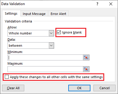
Apart from the validation options, the settings tab also displays two checkboxes:
- Ignore Blank: If this option is marked, it instructs Excel not to validate empty/ blank cells. In technical terms, this option mainly affects the command ‘circle invalid data’. When selected as marked, the cells with no values are not circled even if they fail to pass validation.
- Apply these changes to all other cells with the same settings: If this option is marked, Excel updates the applied validation to all the other cells when there is a match of the original validation of cell/cells being edited.
How to add Data Validation in Excel?
To add a data validation in an Excel sheet, we must perform the following steps:
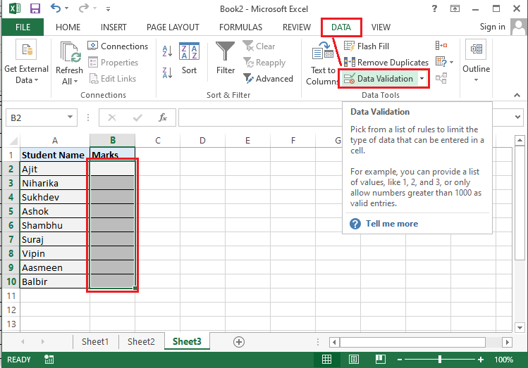
Step 1: Launch the Data Validation dialogue Box
First, we must select all the cells or a range to which we wish to apply validation. Next, we need to navigate the Data tab – Data Tools group and select ‘Data Validation‘ to launch the data validation dialogue box.
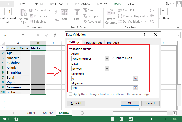
Step 2: Set the Data Validation Rule
After the data validation dialogue box is displayed, we need to go to the Settings tab to define validation criteria. We can provide the desired values, cell references, or formulas in the validation criteria.
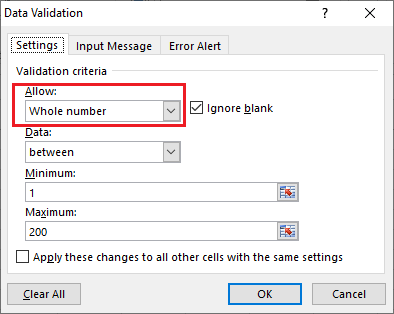
Suppose we need to restrict users to enter marks for each student, but the marks must be supplied in between 0 to 100. This way, we can eliminate the chances of wrong inputs to some extent. For this, we need to set the criteria in the Settings tab as the following image:
After all the validation settings have been set, we need to click the OK button to close the validation dialogue box or move to the next tab to insert an input message and/or error alerts. The other two tabs are optional and used to inform users to enter appropriate values according to the validation rules.
Step 3: Create an Input Message to Display (Optional)
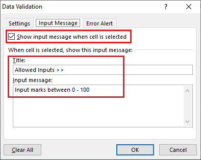
If we want to display a message to the user saying which type of data is supported or allowed in the selected cell, we can use the input message tab. Using the input message, we can inform the user regarding the allowed data type format when the user selects a corresponding cell/ cells.
For example, we can display the following message into the desired fields (cell/cells/range).
Once the input message is entered, we can click the OK button or move to the Error Alert tab further.
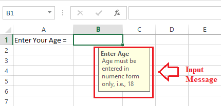
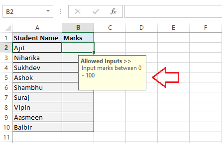
After setting up an input message, the corresponding cell (s) displays the message like this:
Step 4: Add an Error alert (Optional)
In addition to an input message, we can also set an error alert to display when the user enters invalid data into the respective cells. Moreover, we can also add a custom error message.
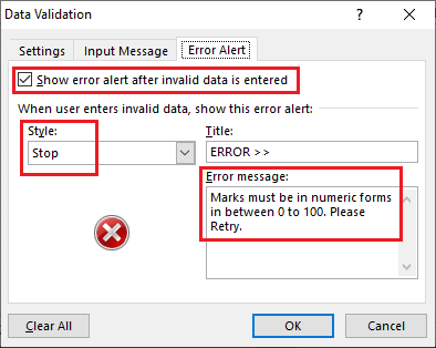
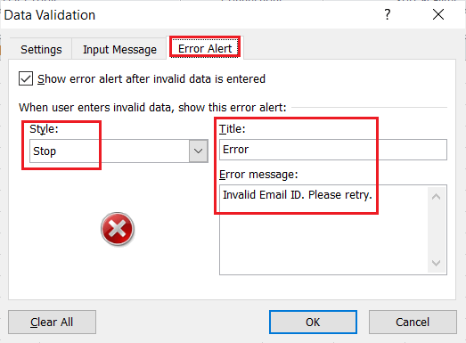
In the above image, we used the option ‘Stop‘ as an error alert style. We can use the other two styles, Warning and Information, accordingly. Lastly, we must click the OK button.
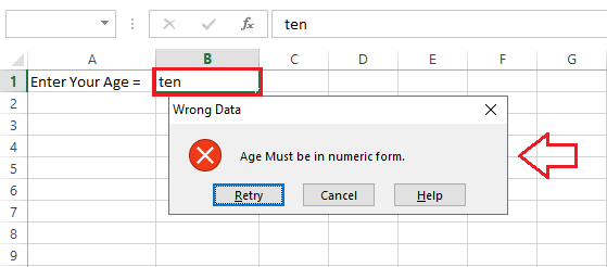
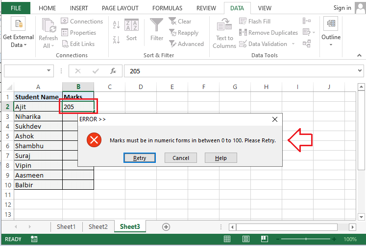
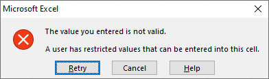
When the user enters invalid data, it triggers an error window with a message, and the invalid input is not allowed.
If we don’t set a custom error alert and set the validation rules ins Excel cell(s), Excel automatically displays the default error alert with the predefined error message. It looks like this:
Data Validation Examples
The following are some essential examples of Data Validation in Excel:
Example 1: Restricting users to enter/choose specified values from the drop-down menu
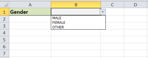
Suppose we want to restrict users to select an option/ value from a list of predefined values. This case of data validation is used in most of the Excel sheets. In our example, we want to restrict users to select a gender from the predefined values, such as ‘MALE’, FEMALE’ or ‘OTHER’.
For this, we need to perform the following steps:
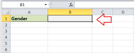
- First, we need to select a cell(s) to apply the validation. In our example, we select cell B1.
- Next, we launch the Data Validation dialogue box by clicking the Data Validation icon under the Data tab on the toolbar.
- After that, we need to choose the List option from the drop-down menu under the Settings tab and specify the list items into the source box separated by a comma. However, if we want to specify several list items, we must refer to a range of cells containing list items instead of entering them directly inside the source box.
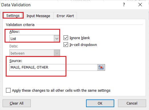
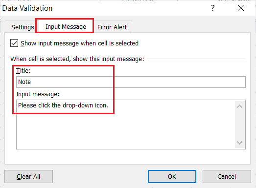
- Lastly, we need to click the OK button. We can also specify the input message from the next tab, as shown in the following images:
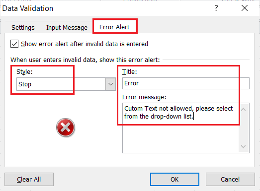
In addition to the input message, we can also specify the error alert message from the next tab:
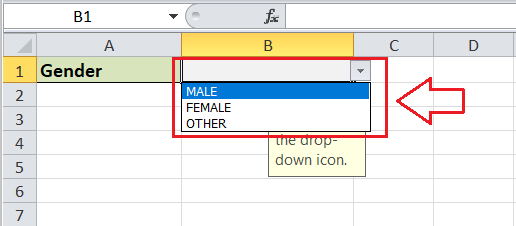
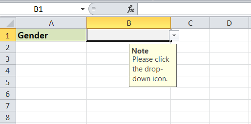
When the user clicks on the restricted cell(s), the drop-down icon is displayed. Users can click the icon to open a list and select the desired option.
When the user clicks on the restricted cell(s), the input message is displayed:
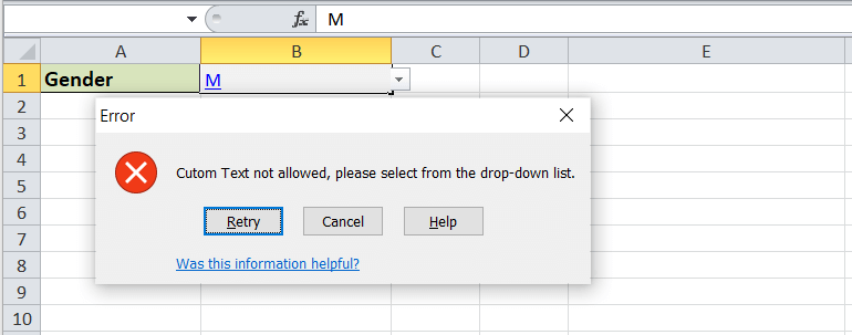
When the user enters the custom text, the error message is displayed:
That is how we can use the data validation feature in Excel and create drop-down lists.
Example 2: Restricting users to enter valid Email Id
Suppose we want to apply data validation in specific cells to restrict users to enter an email id with a valid format, i.e. [email protected], where the domain refers to an email service provider.
For this, we need to perform the following steps:
- First, we need to select a specific cell(s) to apply the data validation. In our case, we select cell B1.
- Next, we need to navigate to the Data tab and select the ‘Data validation‘ option.
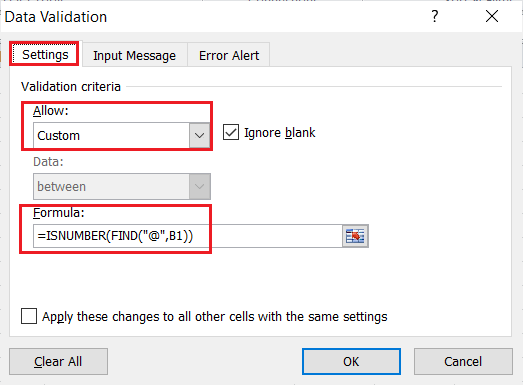
- After that, we need to choose the Custom option from the drop-down menu under the Settings We specify a custom formula “=ISNUMBER(FIND(“@”,B1))” without outer quotes to allow only values with the sign ‘@’ in a selected cell.
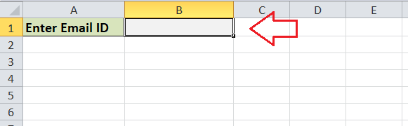
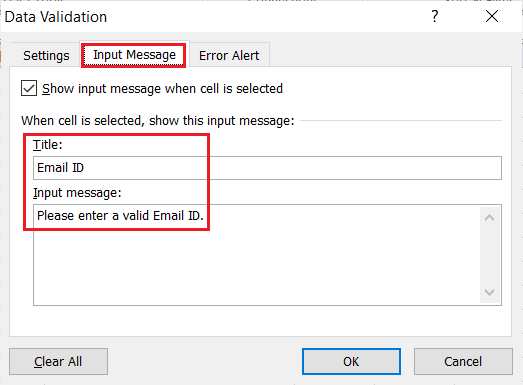
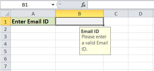
- We can specify the input message to instruct users to enter a valid email id, as shown below:
- Lastly, we must specify the Error alert message, which will only be displayed if a user enters an invalid email id.
- Once all the options are configured in a data validation dialogue box, we need to click the OK button to save the applied changes.
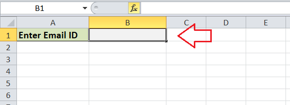
Now, when a user selects the corresponding cell, the input message is displayed:
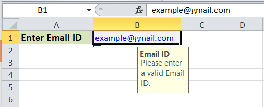
When a user enters a valid email id, it is accepted in a cell after passing the applied validation:
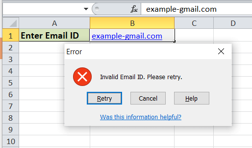
When a user enters an invalid email id, the validation fails and triggers an error alert:
That is how we can restrict specific cells in Excel to accept only the valid email id/ address. Similarly, we can type any other specific text to restrict the user inputs accordingly. However, it is important to note that the FIND function is case sensitive. So, if we don’t need to restrict the case of the text, we can use the SEARCH function instead of the FIND function in the above process.
Example 3: Restricting users from entering future dates
Entering dates in an Excel sheet is one of the common data entry tasks. Sometimes, users may enter wrong dates or future dates, even when all the dates we want in a sheet are recorded earlier. In this case, we can use data validation to prevent future dates in a specific cell(s).
For this, we need to perform the following steps:
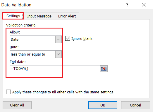
- First, we need to select the specific cell(s) and click the Data Validation icon from the toolbar. We must choose an option Date in a Data Validation dialogue box under the Settings tab. It will display two more sections, such as Date and End Date. Since we want to block future dates, we select the options ‘less than or equal to‘ and put the date formula “=TODAY()” without quotes in corresponding sections.
Once all the validations are set, the Settings tab looks like this:
- After setting the validation rules, we can set an input message and the error alert using the next two tabs similar to what we performed in the above two examples.
Now, when a user selects a respective cell(s), the input message is displayed:
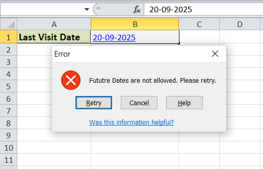
When a user enters a future date, the error alert is displayed:
Similarly, we can allow other restrictions for dates using the Data Validation feature in Excel.
Example 4: Restricting users to enter values of the specified length
Sometimes, there may be cases when we want to restrict users to enter values of any particular length or characters. Suppose there is a need to accept PAN Numbers in cells entered by users. Since the PAN number is a ten-digit unique alphanumeric number, we can create validation rules to accept the values with length 10.
For this, we need to perform the following steps:
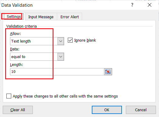
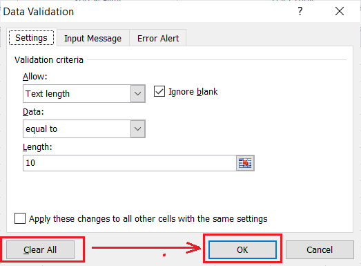
- First, we need to select the specific cell(s) and click the Data Validation icon from the toolbar. We must choose an option Text Length in a Data Validation dialogue box under the Settings tab. It will display two more sections, such as Data and End Length. Since we want to allow 10 digits, we select the options ‘equal to‘ and put the length ‘10‘ without quotes in corresponding sections, respectively.
Once all the validations are set, the Settings tab looks like this:
- After setting the validation rules for a specific text length, we can set an input message and the error alert using the next two tabs.
Now, when a user selects a respective cell(s), the input message is displayed:

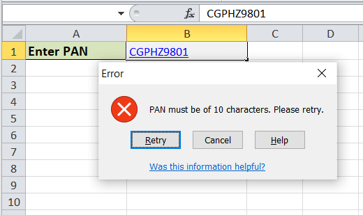
When a user enters a value of less than 10 characters or more than 10 characters, the error alert message is displayed:
Similarly, we can set other restrictions for length based values using the Data Validation feature in Excel.
Example 5: Restricting users to enter values in Uppercase only
If we want to receive user inputs only in uppercase, we can set the validations in Excel. Suppose we want to accept the entry of a PAN number that contains both the text and numbers. However, we only want to take it in uppercase by the user.
For this, we need to perform the following steps:
- First, we need to select the specific cell(s) and click the Data Validation icon from the toolbar. We must choose the option Custom in a Data Validation dialogue box under the Settings tab. Next, we need to apply the custom formula “=EXACT(B1,UPPER(B1))” without quotes. We enter cell B1 in a formula as B1 is the result cell in our example.
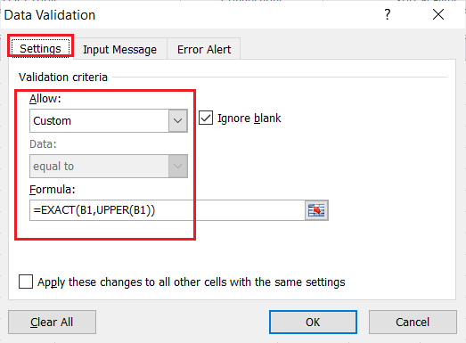
In the above image, the upper function is used to match characters with uppercase. Moreover, the EXACT function ensures that cell entry matches with the uppercase version. - After setting the validation rules for uppercase entries only, we can set an input message and the error alert using the next two tabs.
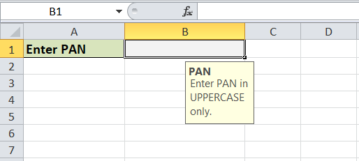
Now, when a user selects a respective cell(s), the input message is displayed:
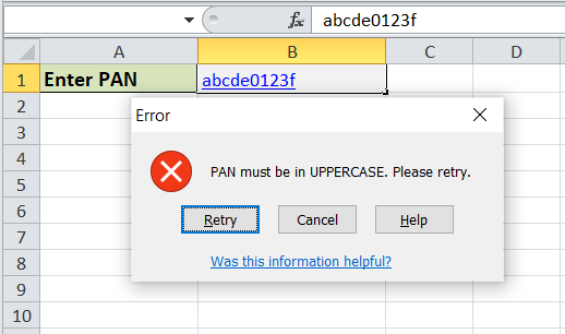
When a user enters an invalid value (value in lowercase), the error alert is displayed:
Similarly, we can set other restrictions with a custom formula using the Data Validation in Excel.
How to edit Validation Rules in Excel?
Suppose we have applied the data validation in an Excel sheet earlier and now edit the validation rules. We must perform the following steps to change or edit the validation rules:
- Select the cells with validation.
- Launch Data Validation Dialog Box from the toolbar.
- Make the desired changes under the corresponding tabs in a dialogue box and click OK.
How to locate or find Data Validation?
Suppose we have an Excel sheet with the data validation rules applied to it. Now, we want to find out the cells with validation. We must perform the following steps to find cells with data validation in Excel:
- Navigate the Home tab on the toolbar.
- Lick the drop-down icon in a shortcut, ‘Find & Select‘ under the ‘Editing’ group.
- Select the ‘Data Validation‘ option from the list.
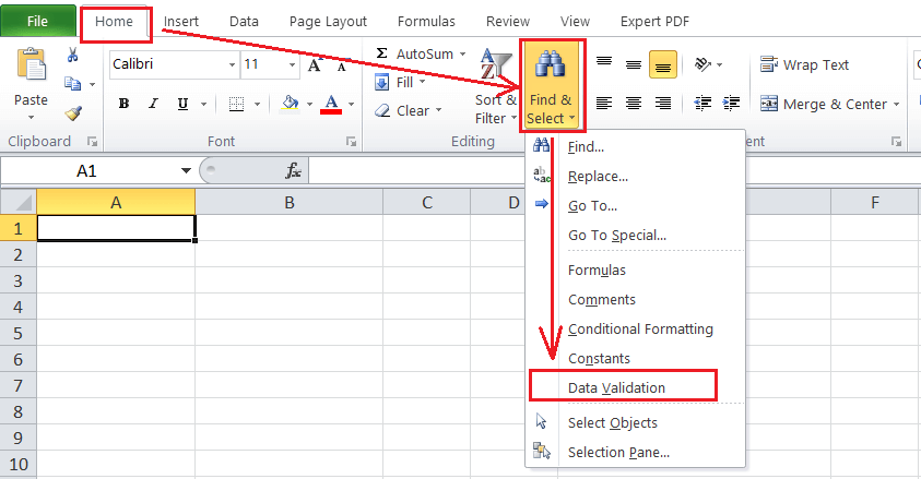
After using the steps, the corresponding cells with the validation will be selected/ highlighted.
How to copy Validation Rules to other cells?
Suppose we have some cells with validation rules, and we want to apply the same validation rules on other cells. To do this, we can use Paste Special feature, as listed below:
- Select and copy the cells with validation using the shortcut Ctrl + C.
- Use the shortcut Ctrl + Alt + V + N to paste the copied cells onto the cells we wish to apply data validation. Alternately, we can launch the paste special dialogue box using the right-click menu options and select the ‘Validation‘ option.
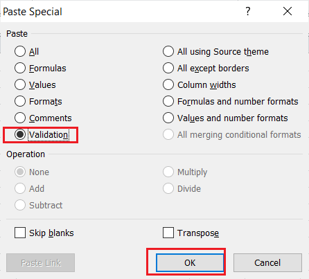
This will apply the same validation on other cells on which the contents are copied.
How to remove or clear Data Validation?
There are two common methods used to remove or clear all the validation in Excel:
Method 1: Clear Data Validation using the Data Validation Dialog Box
- Select all the cells to remove data validation.
- Launch the Data Validation dialogue box from the ribbon.
- Click the option ‘Clear All‘ under the Settings tab and the OK
This will remove/ clear data validation from the selected cell(s).
Method 2: Clear Data Validation using Paste Special Feature
- Select empty cells without validation rules, and copy using the shortcut Ctrl +C.
- Select cell(s) with the validation from which the data validation is to be removed.
- Paste the contents using Ctrl + V and hit Enter
This method typically replaces the data validation with the empty cells, which is an indirect way of removing data validation in Excel.


