

How To Apply Filter In Excel
When the data in MS Excel is too massive to handle, and there is a need to filter the data, then the use of the Filter option is the best one. If we try to manually perform the task, it will consume a high time and may take one whole day. Thus to deal with large data sets, filter is the option. Using filter, we are able to display only those data values that meet certain criteria and hide the other data values. We can apply the filter on text, date or numbers. Also, we can use multiple filters for different columns and narrow the resultant. So, filter can help us filter out the required information and hide the other unwanted information from the datasets.
In this section, we will learn how we can apply filter on a dataset and filter out the necessary data from the entire dataset and display only that portion of the dataset and hiding the unwanted data. We will also know the keyboard shortcut to directly apply the Filter method.
Applying Filter
The purpose of filtering the data is the same, but there are two ways using which we can filter the data. Let’s discuss both the methods one by one.
Method 1
Below are the steps to apply the filter on a given dataset:
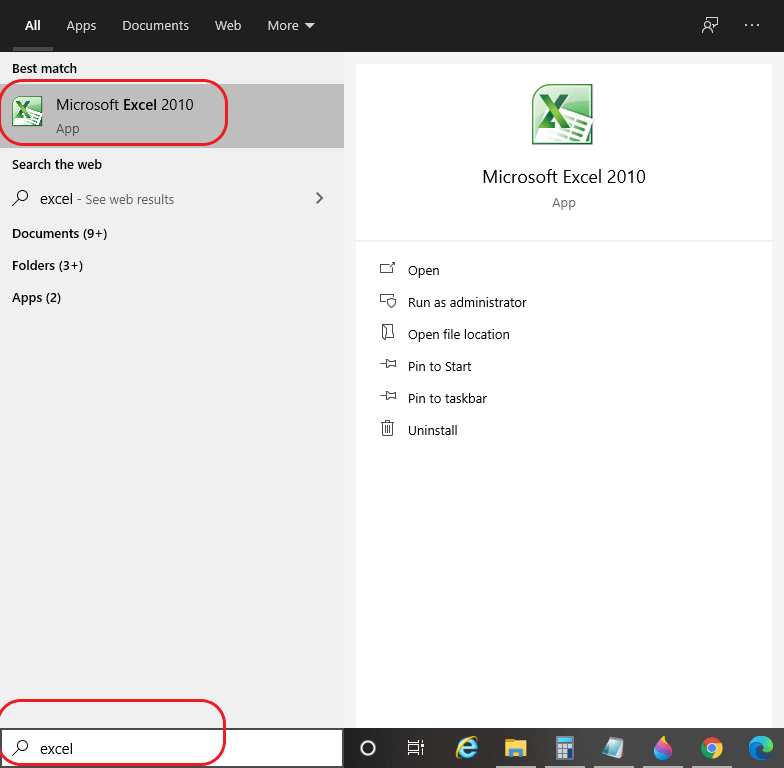
Step 1: Open MS Excel on your computer system either by directly searching on the search tab or using the MS Excel icon, if present on the desktop. A snippet is shown below:

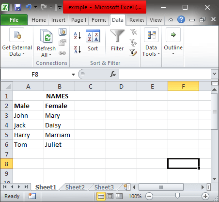
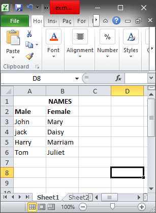
Step 2: Either open an excel file using Ctrl + O and browse for the specific file. Else type out the entire dataset as per your requirement. We have opened an already existing file, as you can see in the below snapshot:
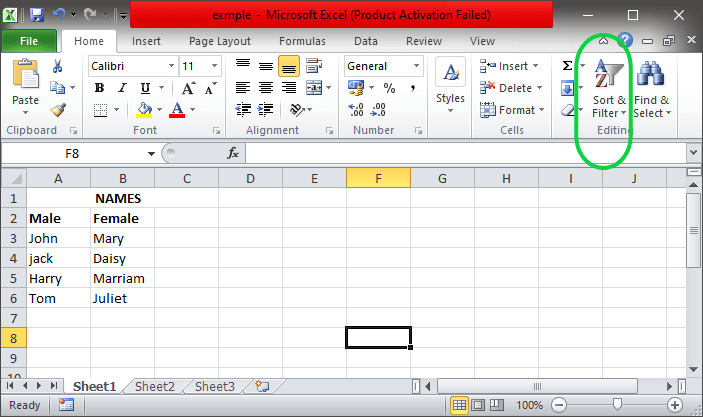
Step 3: On the toolbar, under Home, there are several options from which the last is the Editing section, you can see the Sort & Filter option as you can see in the below snapshot:
Step 4: Select a cell and then click on the Sort & Filter option, and a list of options will appear as shown in the below snapshot:
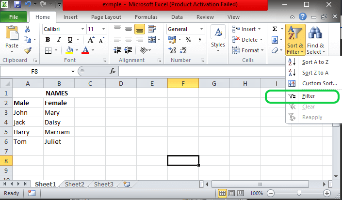
Step 5: Click on Filter from the list.
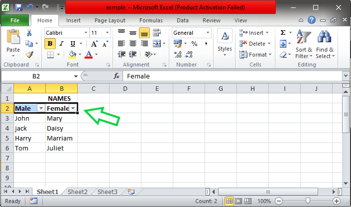
Step 6: Now, a drop-down list will appear on the particular selected row cells, as you can see in the below snapshot:
Step 7: Click on the drop-down list, and a list of options will appear. You will see the below-shown options:
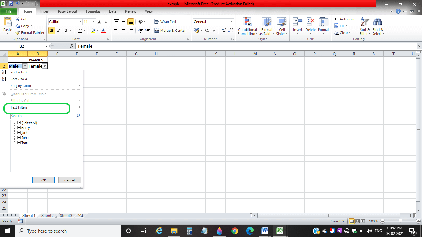
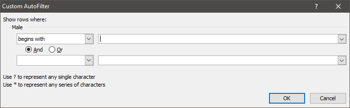
Step 8: Click on Text Filters, and you will see a list of options from which you can select the appropriate filter that you want to apply. For example: For the below-shown dataset, suppose we select Text Filters > Begins With, and the Custom AutoFilter dialog box opens up as shown below:
Step 9: Enter a text for which you want to filter that particular column, which begins with the entered text. Let’s enter ‘M’ in the drop-down box, and below, you can select the condition as AND/OR (select AND if you want to apply two filters; otherwise, select OR if you want to apply anyone filter). So, select the appropriate filter and click on OK as we have performed in the below snapshot:
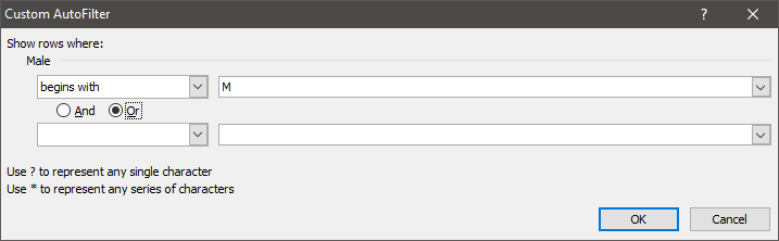
If you don’t want to apply more than one filter, leave it as default.
Step 10: The data as per the applied filter will appear in the worksheet, as you can see in the below snapshot:
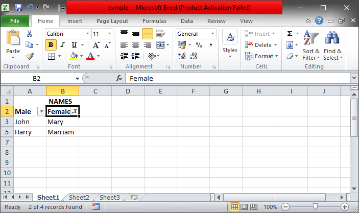
In a similar way, you can apply other filters as it depends on your satisfactory requirements.
Method 2
Below are the steps to apply the filter on the given dataset:
Step 1: Open MS Excel on your computer system either by directly searching on the search tab or using the MS Excel icon, if present on the desktop. A snippet is shown below:
Step 2: Either open an excel file using Ctrl + O and browse for the specific file. Else type out the entire dataset as per your requirement. We have opened an already existing file, as you can see in the below snapshot:
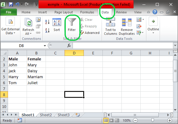
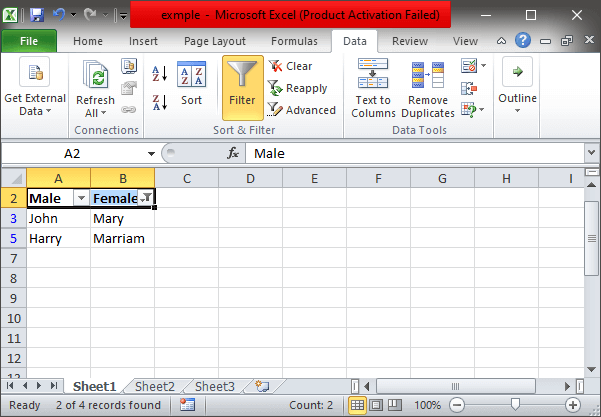
Step 3: On the toolbar, under data, next to Formulas, you will see the Filter icon in Sort & Filter section, as you can see in the below snapshot:
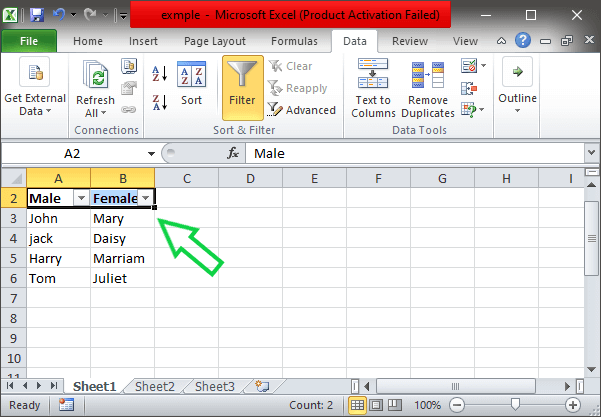
Step 4: Select a cell and then click on Filter, and the drop-down will appear on the selected cell row, as you can see in the below snapshot:
Step 5: Click on the drop-down list, and as per your requirement, you can apply the filter on your data set. The same example can be considered for this method, too, where we have applied the Begins With the filter on the data set, and we got the same result as we got in Method 1, as you can see in the below snapshot:
Therefore, the purpose of the Filter option is the same in both methods. The only difference is the method to access the Filter option.
Keyboard Shortcut
We can also apply the below-described keyboard shortcut for applying the filter to our dataset:
Press Ctrl + Shift +L, and the filter drop-down box will appear on the selected cell row and then follow the same steps and apply the appropriate filter to your dataset.
Point To be Noted:
In the filter dialog box, you will also see the Select All list of options, and you can apply this filter option also as shown below:
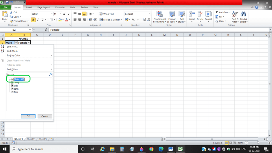
When we used this filter option on our dataset and unselected ‘Tom’ and ‘Jack’ in ‘Male’, we got the following result:
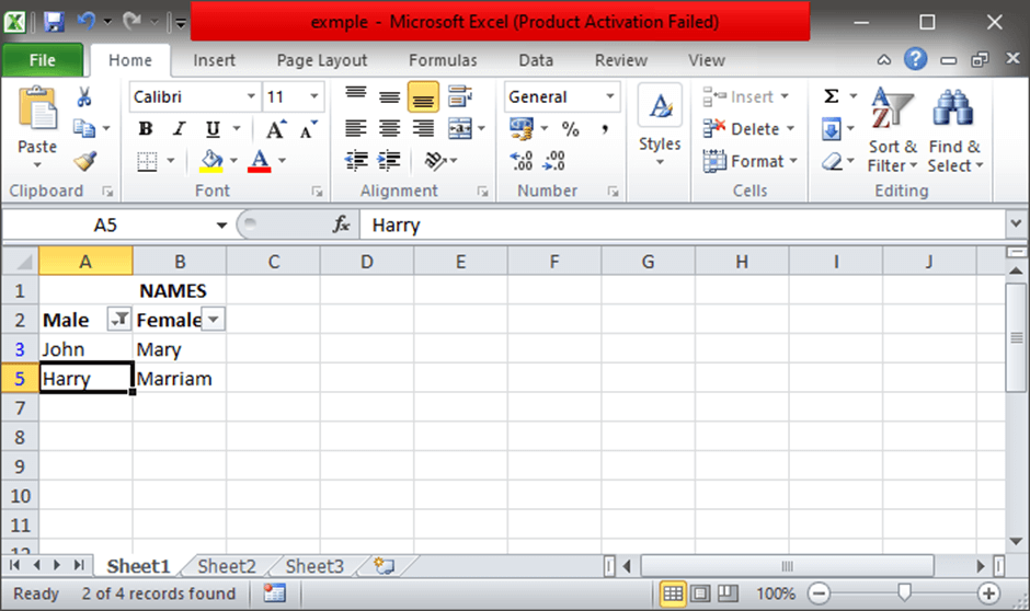
You can notice that on unselecting two names, the data get filtered, and we got the above-displayed data.


