

How to calculate Mean in Excel?
Microsoft Excel (often referred to as Excel) is powerful spreadsheet software designed to store large data sets. Also, it enables users to organize and analyze data and even perform basic to complex calculations on the recorded data. Excel’s essential data analysis tasks mainly include calculating or finding the mean (or arithmetic mean), mode and median.
In this tutorial, we discuss various step-by-step methods or solutions on how to calculate the Mean in Excel. Before discussing the methods, let us first briefly understand the concept of Mean and its benefits.
What is the Mean in Excel?
In Excel, the arithmetic mean is nothing but an average number that is typically calculated by adding all numbers of given data set and then dividing the sum by the total number of values (or count) of given items.
Although it is easy to calculate the arithmetic mean for small data sets in real life, it becomes difficult working with large data sets. That’s where a powerful spreadsheet program like Excel comes in handy. It can easily calculate the Mean of hundreds to thousands of numbers. Also, it is less prone to errors.
There are many essential uses of the Mean in analyzing data, such as:
- To compare historical data
- To highlight KPIs (Key Performance Indicators) and quotes
- To find the midpoint for the given data points
- To determine project management and business plans
The basic scenario when we may need to calculate the Mean in Excel is when we need to find out the average sales of an item in a whole month, quarter, year, etc.
How to calculate Mean in Excel?
Unfortunately, there is no definite MEAN function to calculate or determine the Arithmetic Mean for the data. However, there are a couple of effective ways. Generally, we can usually apply the mathematical concept of adding values and then dividing their sum by the number of values within Excel cells. Furthermore, there are existing functions like AVERAGE, AVERAGEA, AVERAGEIF, and AVERAGEIFS, which also help us calculate the Arithmetic Mean in different use cases.
To get a better idea of how these concepts work for computing the arithmetic mean, let us discuss each one individually with an example:
Calculating Mean in Excel: General Method
We can apply the SUM and COUNT functions in an Excel sheet to use the approach of adding values and dividing them by the number count of included values.
For example, suppose we have given the numbers from 1 to 5 and need to calculate the arithmetic mean. Mathematically, we first add up all these numbers, i.e., (1+2+3+4+5). Afterwards, we divide their SUM by 5 because it is the total count of given numbers.
Thus, the entire formula to calculate the Mean becomes this:
(1+2+3+4+5)/ 5
This returns the arithmetic mean 3.
In Excel, we can use the above mathematical formula by combining it with the SUM and COUNT functions in the following way:
=SUM(1,2,3,4,5)/COUNT(1,2,3,4,5)
Here, the SUM function adds up the given values, while the COUNT function determines the number of given values.
Now, if we record these five numbers in range A1:A5, the below formula in cell A6 will calculate the arithmetic mean:
=SUM(A1:A5)/COUNT(A1:A5)
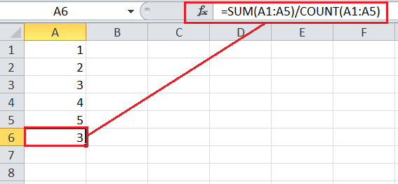
The result (or Mean) obtained in the above image is the same as that we calculated from the mathematical formula, i.e., 3.
Calculating Mean in Excel: AVERAGE Function
Since the Mean is an average, Excel’s AVERAGE function is the most efficient way to calculate the arithmetic mean. It is one most commonly used statistical functions to calculate the Mean for a certain range if there is no special condition or limitation. It is the built-in Excel function.
Syntax
The syntax of Excel’s AVERAGE function is as follows:
=AVERAGE(number1, [number2], …)
The number1 is the required argument, meaning that one argument is mandatory in the AVERAGE function. However, we can supply multiple arguments in different forms like numbers, cells, ranges, arrays, constants, etc. When calculating the Arithmetic Mean, we should supply at least two arguments in the AVERAGE function.
Steps to Calculate Mean using the AVERAGE Function
Let us now understand the working of the AVERAGE function and calculate the arithmetic mean for a group of numbers in an Excel sheet using the sample data.
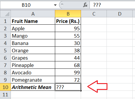
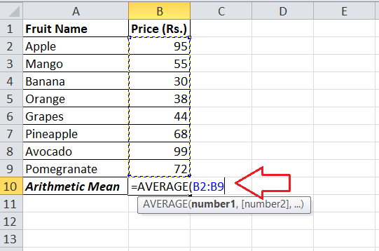
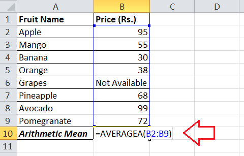
Suppose we list some fruits in an Excel sheet with their corresponding prices. The fruit names are recorded in column A (A2:A9), and their prices are in the following column B (B2:B9). We need to find or calculate the average price (or arithmetic mean for the prices) in cell B10.
We need to perform the below steps to calculate the arithmetic mean in our example worksheet:
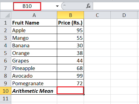
- First, we must select or highlight the cell to record the resultant arithmetic mean, i.e., cell B10.

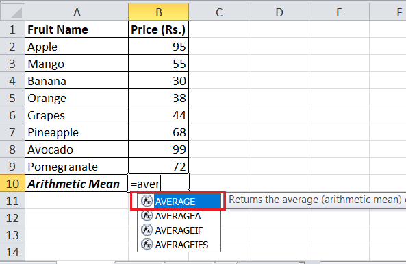
- Next, we need to insert the function name starting with an equal sign and provide the necessary arguments in the function. In our case, we type the equal sign (=) and the AVERAGE function. We can also choose the function from the list of functions suggested by Excel.
- After entering the function name, we must enter the starting parenthesis and supply our effective range of data sets. Since we have data in adjacent cells or a range (from B2 to B9), we can pass the entire range in the function in the following way:
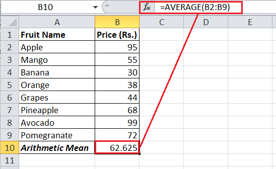
- Lastly, we must enter the closing parenthesis and press the Enter key on the keyboard to get the effective result or Arithmetic Mean for the given data set. The below image shows the arithmetic mean for the prices in cells from B2 to B9:
In the above image, we used the adjacent cells and supplied the entire range of data sets in one go. However, we can also calculate the Mean for the non-adjacent cells in our Excel sheet by supplying the cells individually.
Suppose we only need to calculate the arithmetic mean of prices for only three fruits: Apple, Mango, and Grapes. In that case, we can pass each cell separately in the function in the following way:
=AVERAGE(B2,B3,B6)
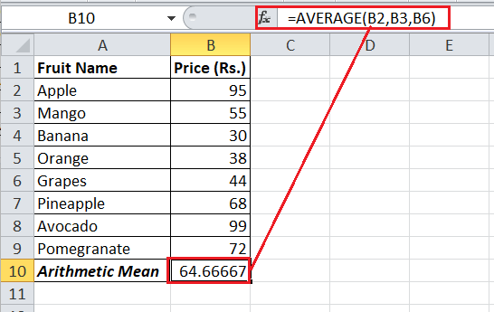
Here, B2, B3, and B6 are the individual cells with the prices of Apple, Mango and Grapes.
Although the AVERAGE function can be used with empty cells, texts, zeros, logical values and even mixed arguments, it ignores the empty cells, text and logical values during the calculation. However, the zero-value cells are included in the AVERAGE function.
Calculating Mean in Excel: AVERAGEA Function
The AVERAGEA function is a slightly advanced version of the AVERAGE function. The AVERAGEA function also helps us calculate the arithmetic mean for given data sets and works in all versions of Excel. One benefit of the AVERAGEA function is that it can include text values and the Boolean data types while calculating the Mean in Excel. The text values are evaluated as zeros, while the Boolean values TRUE and FALSE are evaluated as 1 and 0, respectively.
Syntax
The syntax of Excel’s AVERAGEA function is as follows:
=AVERAGEA(value1, [value2], …)
Like the AVERAGE function, the first argument in the AVERAGEA function is required. However, we can use multiple arguments as needed.
The syntax of the AVERAGE and AVERAGEA functions are almost similar; however, their working concept is slightly different. The AVERAGE function can only calculate the arithmetic mean for numeric values, while the AVERAGEA function can calculate the same for any data type, including text and Booleans.
Steps to Calculate Mean using the AVERAGEA Function
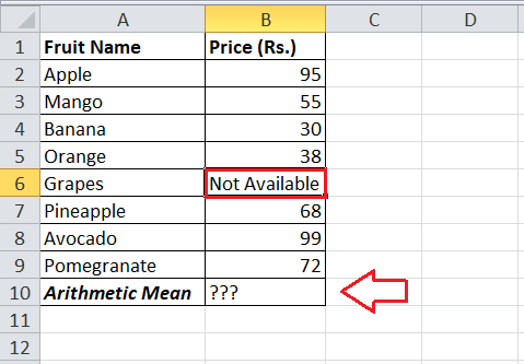
Let us retake the previous example data sets where we have fruit names in column A (A2:A9) and their prices in column B (B2:B9). However, we don’t have the price for the Grapes this time (recorded as ‘Not Available’ in the corresponding cell B6), as shown below:
We can execute the below steps and calculate the mean value using the AVERAGEA function:
- Like the previous method, we first select the resultant cell B10 to record the Mean. Next, we type the equal sign (=), enter or select our function AVERAGEA, and pass the entire data range to the function enclosed within the parenthesis.
- Lastly, we must press the Enter key to obtain effective output (or mean).
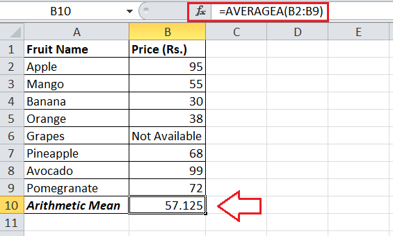
The above image returns the mean output of 57.125 with the AVERAGEA function.
If we use the AVERAGE function in this example and calculate the arithmetic mean, we see a huge difference between the results obtained by both functions. The mean output of 65.285 appears with the AVERAGE function, as shown below:
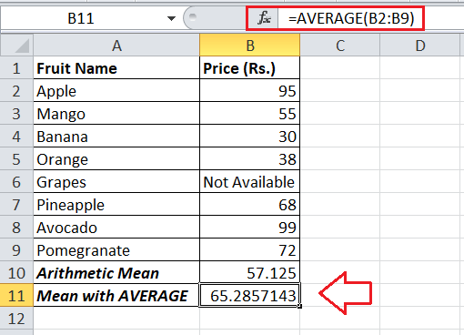
The differences in Arithmetic Mean in this example makes sense because the division count number is different for both these functions. The number count for the AVERAGEA function is 8, as it also evaluates the TEXT as valid data. But, for the AVERAGE function, the division count is 7 since it does not include the TEXT data in its calculation.
Instead of TEXT data, if the data set contains zero (0), the same result (or arithmetic means) will appear for both functions (AVERAGE and AVERAGEA) because both include zero as valid data in the calculation.
Calculating Mean in Excel: AVERAGEIF Function
The AVERAGEIF function is the relevant function of the AVERAGE function and helps us calculate the arithmetic mean with a given condition or criteria. With the AVERAGEIF function, we can only calculate the Mean for certain numbers that follow the specified criteria. Excel first evaluates the specific criteria, locates the effective cells following those criteria and then calculates the Mean for only the located cells accordingly.
Syntax
The syntax of Excel’s AVERAGEIF function is as follows:
=AVERAGEAIF(range, criteria, [average_range])
Here, the range and criteria are the required arguments, while the average_range is optional.
- A range contains cells to be tested against the given criteria.
- A criteria refers to the argument where we can specify the desired condition to follow. It can include text, numeric values, cells reference, range, and logical expression.
- The average_range is the argument where we mention cells (or a range) for which we want to calculate the Mean. If this argument is not specified, Excel uses the range automatically.
Steps to Calculate Mean using the AVERAGEIF Function
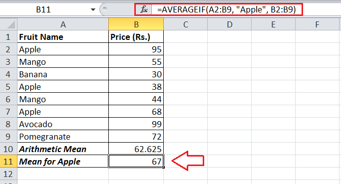
In the same example, suppose we list some fruits multiple times with different prices. This time, we only need to calculate the Mean for any specific repeated fruit (i.e., Apple) in cell B11. So, we use the AVERAGEIF function and apply the condition while calculating the Mean. We must execute the below steps to calculate the Mean price for Apple:
- First, we select the resultant cell (B11) and insert the AVERAGEIF formula in the following way:
=AVERAGEIF(A2:B9, “Apple”, B2:B9)
Here, A2:B9 represents the effective range, Apple represents our desired criteria/condition, and B2:B9 represents the average_range.
Here, we supplied the optional average_range manually to include only the cells with the prices. In our example, if we don’t pass the average_range, the function will use the primary range (A2:B9) with the text data and cause the #DIV! error.
Note: It is essential to note that the AVERAGEIF function ignores the blank cells in its argument average_range. Additionally, if any cell specified in the criteria is blank, the function treats it as a zero-value cell.
Calculating Mean in Excel: AVERAGEIFS Function
The AVERAGEIFS function is an extended or advanced version of the AVERAGEIF function. The AVERAGEIF function only allows us to apply one condition at a time. However, with the AVERAGEIFS function, we can apply multiple criteria to be tested simultaneously. Additionally, the AVERAGEIFS function enables us to use cells with Boolean TRUE and FALSE values, helping us test multiple criteria easily. This is also not possible with the AVERAGEIF function.
Syntax
The syntax of Excel’s AVERAGEIFS function is as follows:
=AVERAGEAIFS(average_range, criteria1_range1, criteria1, [criteria2_range2, criteria2], …)
Here, the average_range, criteria1_range1 and criteria1 are the required arguments. However, we can supply the optional arguments based on our effective data sets. Furthermore, criteria1 refers to a condition to be tested on range1, criteria2 refers to a condition to be tested on range2, and more.
Steps to Calculate Mean using the AVERAGEIFS Function
Let’s consider the same example data we used in the previous method. In the previous method, we used the AVERAGEIF function and calculated the Mean for the prices of repeated fruit (Apple). In that case, we had only one condition.
Now, suppose we have to calculate the Mean for the prices of Apple but only include those cells where prices are above 40.
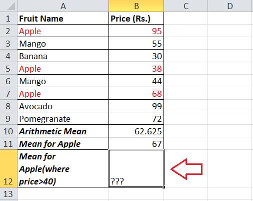
We have two different criteria in this case, so the AVERAGEIF function cannot be used.
Criteria1: In a range A2:A9, the initial criteria is to check for ‘Apple’ that is satisfied by three cells (or rows)
Criteria2: In a range B2:B9, the other criteria is to check for prices above 40 (>40) that is satisfied by the two out of three cells (or row) with a fruit Apple
Thus, if we mathematically calculate the Mean, we use the below formula:
(95+68)/2
This returns the mean value of 81.5. Let’s check if we get the same results with the AVERAGEIFS function in Excel.
When we need to test conditions in Excel, we usually take the help of the OR logical operator. The OR operator returns TRUE and FALSE depending on whether the given condition satisfies. For example, suppose we need to check if cell A2 contains Apple. In this case, we can use the OR operator like this:
=OR(A2=”Apple”)
We insert the above condition in our example sheet to test or locate cells with the fruit Apple. So, we create a new column (C) and type the specific condition in cell C2. Afterwards, we copy down the same condition in the remaining cells of column C. It looks like this:
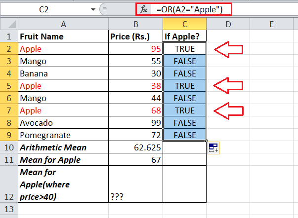
The above image shows that the OR operator returns TRUE for cells corresponding with the fruit Apple, while for others, it returns FALSE. Based on this result, we now apply the AVERAGEIFS function and insert multiple conditions for TRUE value cells in the following way:
- Like other methods, we again first select the resultant cell (i.e., B12).
- Next, we enter the AVERAGEIFS formula in the following way:
=AVERAGEIFS(B2:B9,C2:C9,”TRUE”,B2:B9,”>40″)
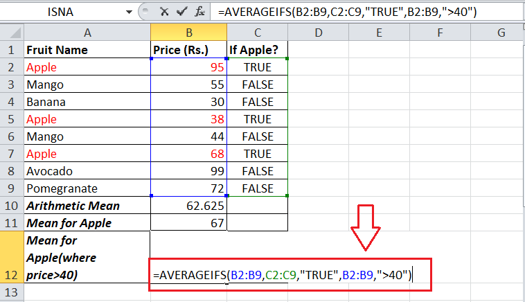
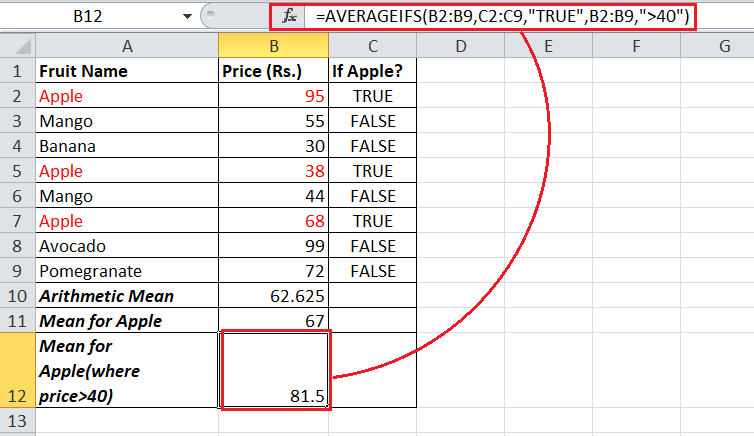
With the above AVERAGEIFS formula, we only included the fruit ‘Apple’ and prices above 40. - Lastly, we must press the Enter key to obtain the formula result. For our dataset, the formula returned the arithmetic mean of 81.5, the same as our mathematically calculated result.
Special Cases
Although we may have various scenarios while calculating the arithmetic mean in Excel, the two most common ones are discussed here. We must be cautious when computing the arithmetic mean in these cases.
Calculating Mean Including Zeros
When we need to compute the Mean with the zeros, we can normally use the AVERAGE function and supply the effective cells, including the zero value cells. The AVERAGE function includes the zeros as valid numbers in its calculation.
In the following sample dataset, we apply the AVERAGE function to calculate the Mean for two different students’ marks:
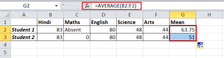
The above image shows the different mean values for both students. If we look at the marks, the sum of marks is the same for both students. The second student has zero marks in one subject (zero value cell), while the first student is absent (text value cell) in one subject.
Since the AVERAGE function ignores text values but includes zero values, the division count varies for both students. For the first student, the division count is 4, while for another student, it is 5. Thus, there is a difference in mean results. However, we can also explicitly exclude zero values if needed.
Calculating Mean Excluding Zeros
When we need to compute the Mean excluding the zeros, we must take advantage of Excel’s AVERAGEIF function. We can apply the specific condition in this function, instructing Excel not to include the zero value cells during calculation.
The below AVERAGEIF formula can be used to exclude zero values while calculating the Mean in Excel:
=AVERAGEIF(cell or a range,”>0″)
If we insert the above formula for our sample data, the same mean value results appear for both students.
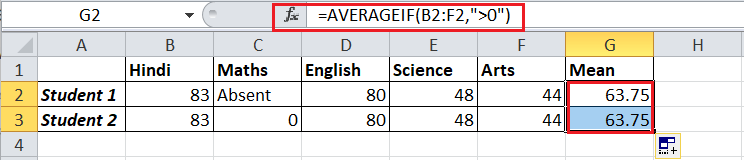
The above AVERAGEIF formula ignores the text and zero value cells. So, the division counts are the same (i.e., 4), and so is the arithmetic mean for the marks of both students.
Important Points to Remember
- It is important to note that any function in Excel, including AVERAGE, AVERAGEA, AVERAGEIF, and AVERAGEIFS, can accept a maximum of 255 arguments.
- Manually typing the function name in an Excel cell is not recommended. Selecting the desired function from the suggestion list is better to avoid misspelt function names and eliminate errors in the results.


