How to create a Pivot Table in Excel?

MS Excel, usually called Excel, is powerful spreadsheet software designed to store considerably huge data sets across worksheets within the cells. A Pivot Table is Excel’s most valuable built-in tool when dealing with extensive amounts of data because it helps us make such data sets more manageable and meaningful for analyses.

A Pivot Table refers to an existing feature in Excel that enables users to extract or represent data in a preferred format (such as customized reports or dashboards) from comparatively large data sets in the same or different worksheets. In particular, it allows users to summarize, sort, filter, and group desired data differently while performing other complex calculations at the same time.

In this tutorial, we discuss essential methods or solutions on how to create a Pivot Table in Excel. Before learning the process of creating a Pivot Table in the worksheets, we must know its core components.

Note: We must not be confused between the terms ‘PivotTable’ and ‘Pivot Table’. Both these terms are interchangeably used. However, the Pivot Chart is an entirely different thing or feature of Excel.

Basic Components of an Excel Pivot Table

Before we learn how to create a Pivot Table within an Excel worksheet, we must know the basic components that help form the Pivot Table. They are:

Pivot Cache: When we try to create a pivot table using certain data sets, Excel automatically creates a snapshot of the given data and temporarily stores it in memory to speed up or smooth out the performance. This snapshot is commonly referred to as the Pivot Cache. One drawback of Pivot Cache is that it does not refresh itself when we add/insert new data into the source table. We have to manually refresh the pivot table to update the pivot cache every time new data is inserted into the source.

Values Area: The values area is used to specify the calculation data.

Rows Area: The rows area is used to specify the headings on the left of the Values area.

Columns Area: The columns area is used to specify the headings at the top of the Values area.

Filters Area: The Filters area is used to go deeper into the data set and view specific data more preciously. However, it is not mandatory.

Methods to create a Pivot Table in Excel

Excel provides several methods to perform any specific task or operation. Similarly, we can create a pivot table in an Excel worksheet using various methods. The two most common ways to insert or create a pivot table in Excel are discussed below:

Method 1: Creating a Pivot Table using the Ribbon

Creating a pivot table using the tools on the Ribbon is the most commonly used method in Excel. However, we must initially prepare or organize the data properly within the sheet. We can select any cell, range, or table structure in the sheet to create our pivot table accordingly. Before we begin, we must ensure that our data has a row header at the top and that there are no empty rows or columns between the data sets. Moreover, if we format our data as a table, it will be very easy to create a proper pivot table.

Suppose we have the following sample data in an Excel worksheet. The data is formatted as a proper Excel table and contains 17 records, including the five fields of information: Date, Color, Region, Units, and Sales.

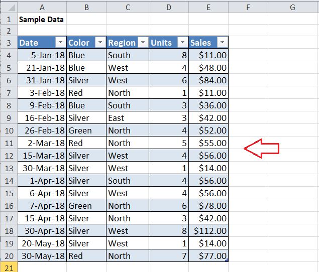
Note: Any data set in an Excel sheet can be formatted as a table by navigating to the Insert tab > Table. However, the effective data range should have already been selected before clicking on the Table option.

The following are the steps to use the above sample data and create a Pivot Table accordingly:

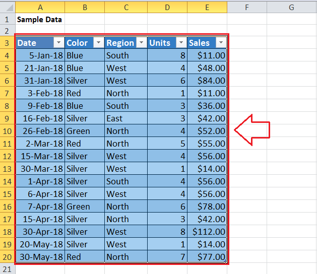
• First, we must select the entire data range we want to include in our Pivot Table. We can also select any single cell of the respective range and supply the entire data set in the later steps.
  
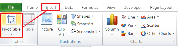
• After selecting the effective data range, we must navigate the Insert tab on the Ribbon and click on the ‘PivotTable’ button. Clicking this button will launch another window named ‘Create PivotTable’.
  
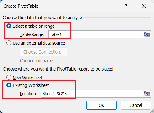
• In the next window, our selected data range is automatically prefilled, which is Table1. However, we can also type or select the range using the box next to the ‘Table/Range’ option under the ‘Select a table or range’ section. Also, we must choose to create a Pivot Table in the new worksheet or the same (existing) worksheet. In our case, we select the same sheet option to compare the source data and Pivot Table side by side. We must also select a cell to start the Pivot Table if we choose the ‘Existing Worksheet’ option.
  
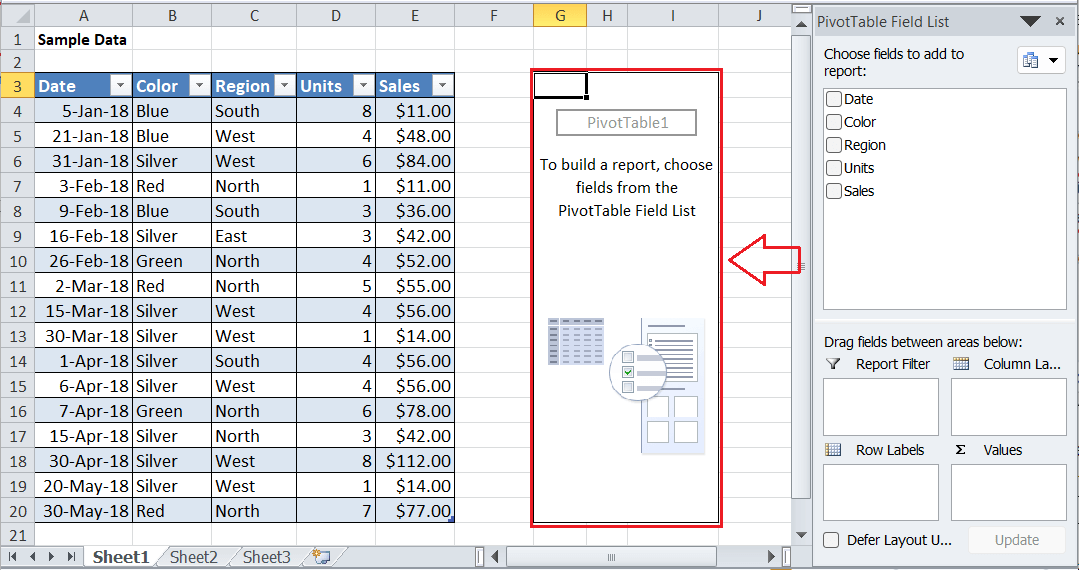
• After giving the input or source range and the destination location for the Pivot Table, we must click the OK button. This will immediately insert or create an empty Pivot Table in the selected location, as shown below:
  
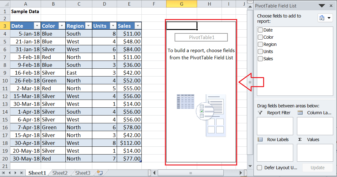
  The above image shows the blank Pivot Table in the existing worksheet and a side pane to the right. We can see the names of all the fields in the side pane, meaning all the fields from the selected range have been extracted. However, we must add or drag the desired fields into the given areas/boxes like Column Labels, Row Labels, or Values accordingly.

Method 2: Creating a Pivot Table using the Keyboard Shortcut

Another common way to perform most Excel tasks is through keyboard shortcuts. Excel has many built-in shortcuts, and we can create or modify new keyboard shortcuts accordingly. We can use the Alt key method if there is no predefined shortcut for an Excel feature but if it is present on the Ribbon. Accordingly, we must first press the Alt key and then press the other displayed keys in a sequence. We can use the keyboard shortcut ‘Alt + D + P’ to access the pivot table feature.

To create a pivot table, let’s look at the same sample data again. To use keyboard shortcuts and create a corresponding pivot table, we need to follow the below steps:

• As in the previous method, we first need to select the data we want to include in our pivot table. Alternatively, we can select one or more cells in the effective data range and proceed to the next step. In this case, we have to supply the desired data range later.
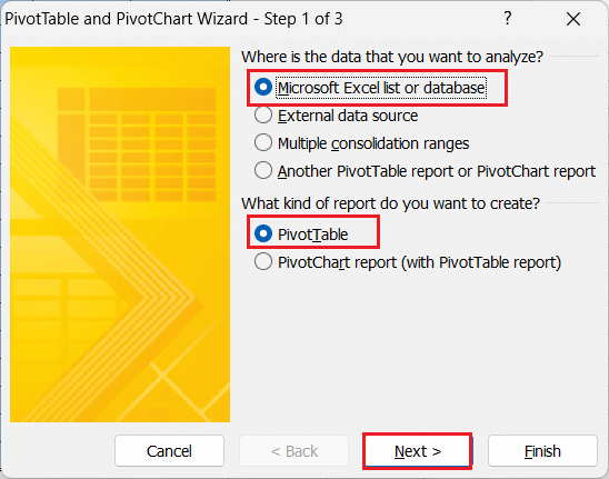
• Next, we have to press the Alt key followed by the D and P keys in a sequence one after another. This immediately opens another window named ‘PivotTable and PivotChart Wizard’.
  
• In the next window, we have to select the first circle radio button associated with the ‘Microsoft Excel list or database’ option as we have our source data in an Excel sheet. Also, we must choose the ‘PivotTable’ option in the below section and click on the ‘Next’ button.
  
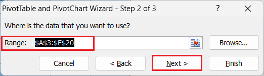
• In the next step, we need to supply the range of cells where our data exist. Since we have already selected the data in the first step, our effective data range is prefilled automatically. However, we can change the range accordingly if needed. After that, we must click the ‘Next’ button again.
  
• In the next screen, we need to tell Excel where to create our Pivot Table. We can choose between the ‘New Worksheet’ and ‘Existing Worksheet’ as the previous method. If we select the same sheet to create a Pivot Table, we must supply or select the sheet’s cell to start Pivot Table and click on the ‘Finish’ button.
  
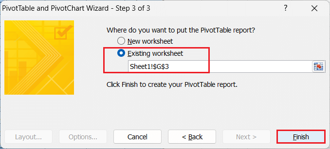
• After we click the ‘Finish’ button, an empty Pivot Table appears that starts from the entered or given cell address in the same sheet, as shown below:
  
  Like the previous method, the Pivot Table is blank, but we have all the field names listed in the side pane. We must modify or add the desired field to the Pivot Table to make it effective.

Modifying/ Arranging the Pivot Table in Excel

After inserting the blank/empty pivot table in the excel sheet, we should add the desired fields and arrange the content accordingly to make it useful. Some of the common adjustments that we need to make frequently are discussed below:

Adding/ Dragging Data to Pivot Table

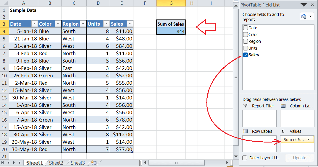
A pivot table is not useful until we know how to appropriately add or drag the desired fields into specific areas/ boxes. For example, we can drag the ‘Sales’ field to the ‘Values’ box in the side pane to know or view the total sales. It simply creates a small Pivot Table summarizing total sales, as shown below:

Since the Pivot Table allows us to add more than one field in an Excel worksheet, we can get more data statistics in a summarized way from our source data. Suppose we want to view the separated sales based on their colors. In that case, we must drag another field named ‘Color’ into the ‘Rows’ box. This makes it easier to determine the highest and the lowest sales for specific colors.

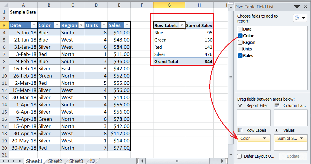
In the above image, we can change the title ‘Row Labels’ to ‘Color’ to make the pivot table more meaningful. If we compare the last two images, the total sales in both remain the same. By adding one more field, we have only split the sales data by colors while the sales remain intact.

Editing the Pivot Table Title

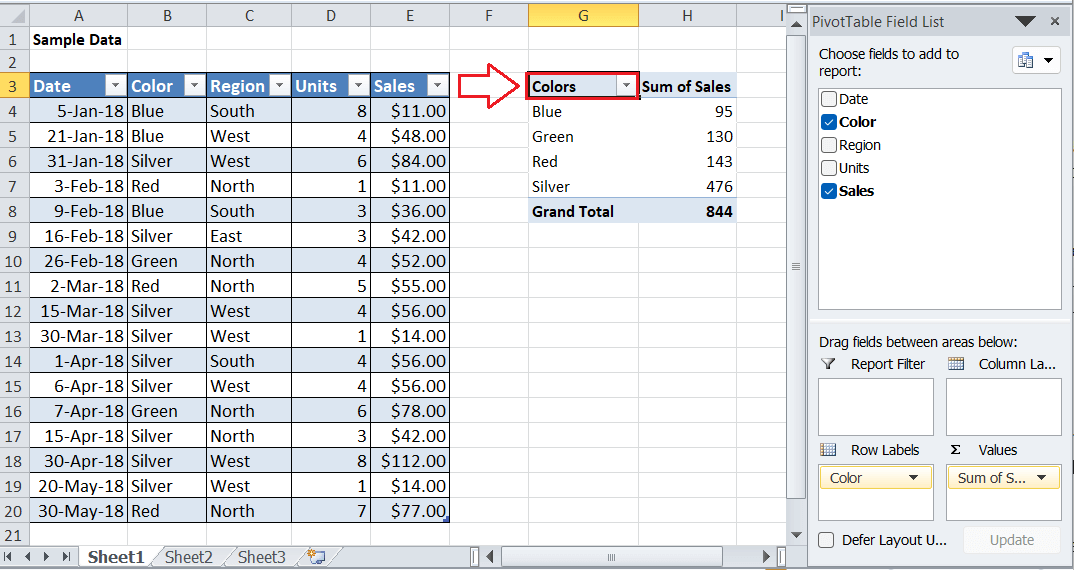
By default, Excel automatically places headings or titles within pivot tables. However, it also allows us to modify the headings accordingly. To modify headings in a pivot table, we need to click on a cell or title and start typing the new desired title. This is similar to editing other content in an Excel cell.

In the image below, we change the ‘Row Labels’ title and enter our custom title ‘Colors’:

Refreshing the Pivot Table

Refreshing the pivot table is required when we add, edit or remove any data in the source table or range. This is necessary to update the pivot cache and bring changes accordingly in our inserted pivot table.

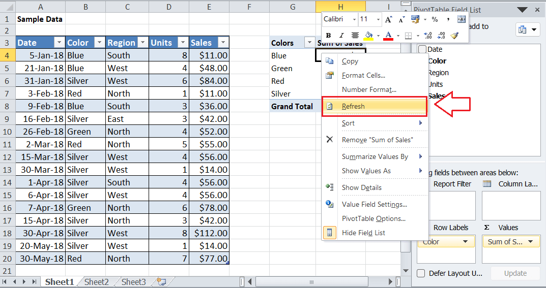
To refresh the Pivot Table, we must press the right-click button on any cell in the Pivot Table and click on the ‘Refresh’ button in the contextual menu. All the data within the table is updated immediately based on the source data.

Formatting Numbers in Pivot Table

As with normal Excel sheet data, we can adjust the number formatting for pivot table data while maintaining the same numerical fields as the source data. For example, our sample data shows a currency symbol ($) in sales data that is not in our pivot table. Therefore, we must manually adjust the number formatting in our pivot table.

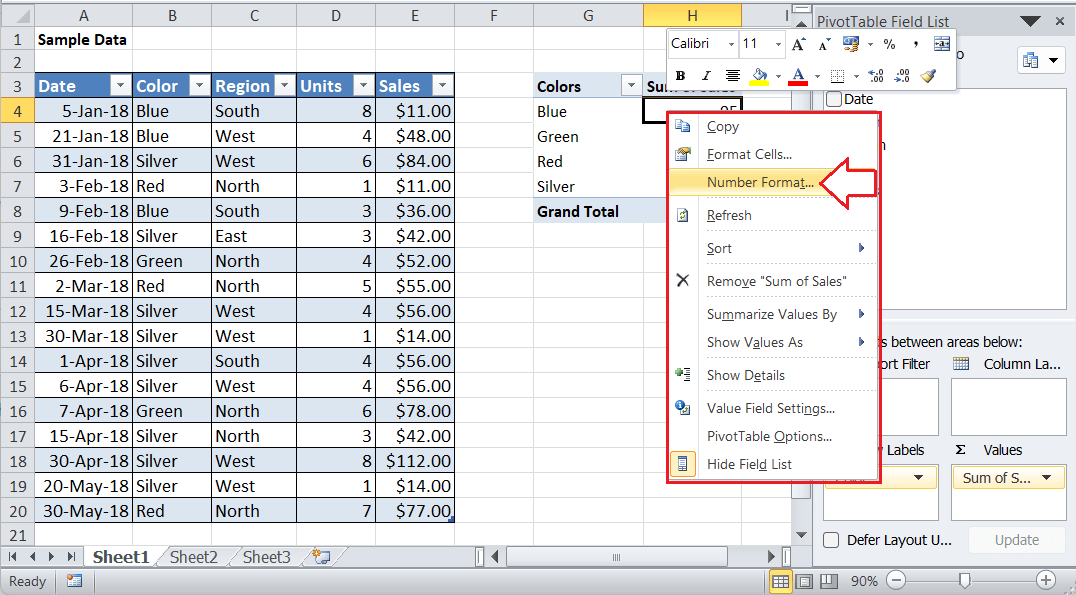
We must press a right-click button on any sales cell in our Pivot Table and select the ‘Number Format’ option in the list.

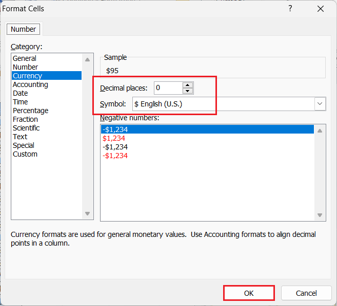
This will open the ‘Format Cells’ window where we need to go to the ‘Currency’ section and select a Dollar ($) next to the Symbol box. Also, we can adjust the decimal places for the numbers accordingly. After making changes, we must click the OK button, and changes will be applied instantly.

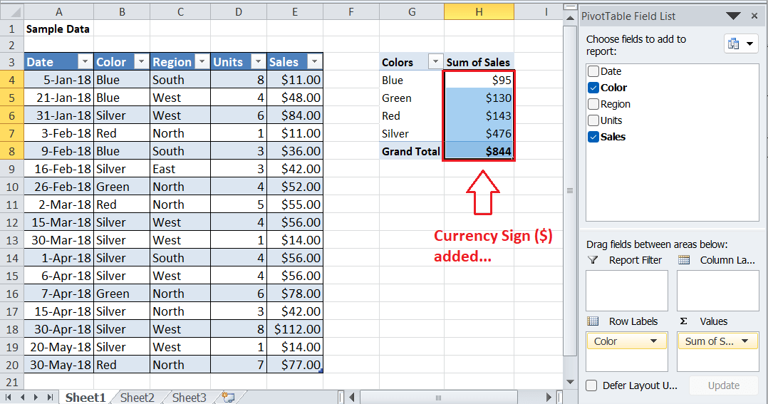
After applying the desired preferences for numbers, Excel will continue to serve the same preferences regardless of changes to the source data or rearrangements in the table.

Sorting and Filtering the Pivot Table

Sorting and Filtering are essential features of Excel. We can also use both these features with our Pivot Table. We can sort the data from ‘highest to lowest’ or ‘lowest to highest’ whenever needed. Similarly, we can apply or insert filters at the top level in our table.

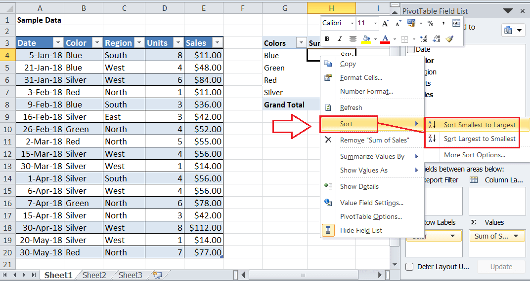
To sort the data in our pivot table, we must right-click on any sales cell and select the ‘Sort’ option in the list. After that, we can choose between sorting options, such as ‘smallest to largest’ and ‘largest to smallest’.

To apply filters to our pivot table, we must drag the desired field to the Filter box in the side pane. The selected field will be added to the top, and a filter icon/button will be displayed.

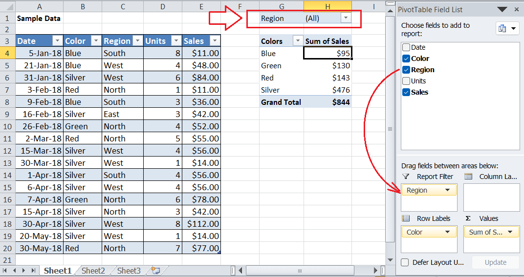
We must click the Filter button and select the desired filtering options accordingly.

Important Points to Remember

• Instead of creating our customized Pivot Tables, we can choose between a few recommended options. Once the useful data for the Pivot Table is selected, we can navigate the Insert tab and click on the ‘Recommended PivotTables’ button under the section ‘Tables’. It will show some suggestions, and we can select any Pivot Table that fits our purpose.
• We cannot interchange the terms ‘PivotTable’ and ‘PivotChart’. Both are different. A Pivot Table enables us to display a summarized view of large data set as per our requirements. At the same time, the Pivot Chart is the graphical representation of the Pivot Table data.