Pie Chart

Pie charts are one of the common elements that are used a lot in Excel worksheets to represent official data. They might seem easy, but there are a lot more things you should know about them to represent your data in a detailed and professional manner that can add value for the reader/clients/management.

What are Pie Charts?

A pie chart is defined as a circular chart with multiple divisions where each division shows the contribution of each value to the total value. The Pie (or the circle) represents the total value, i.e., 100 percent, and each slice of the pie chart adds some per cent to the total.

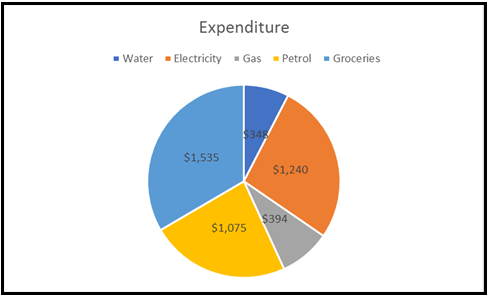
Pie charts usually represent the data where the values can be added together or with only one data series (all the data points are positive). For instance, in the above example, we have created a pie chart to represent the expenditure list of an xyz company. The company has 5 different attributes, and therefore the pie chart shows 5 divisions (also known as slices of a Pie).

The larger the contribution of an attribute, the larger will be the size of the slice of the pie chart. A pie chart can be easily interpreted if data points are less (around 7). With more data points, you will have more slices, and some of them would be very small, making the graph difficult to read/interpret.

Advantages of Pie Charts

1. Easy to create: Though most Excel charts are easy to create, trust me, Pie charts are the easiest of them all. With Pie charts, you need not worry about customization and formatting of your chart as most of the time, the default settings are good enough.

Note: There are various formatting options available as well if you want to format your chart.

2. Easy to read: Pie charts are easy to see and therefore can be read easily if you only have a few data points.

3. Management is obsessed with Pie Charts: As per survey, it is reported that managers/clients love to have Pie charts in the official presentation.

Disadvantages of Pie Charts

1. Pie Charts are useful with fewer data points and often becomes complex when adding more data points.
2. Pie Charts can’t be used to show a trend as they are meant to present you the snap of the values at a certain point in time.
3. Pie Charts can’t show multiple types of data values.
4. Pie Charts the difference in data points is minor, you may find it challenging to comprehend the pie chart visually.
5. Pie Charts take more space and give less information.

Types of Pie Charts

In Excel, there are different types to represent your PIE charts. To access its various types go to the charts group and select Pie chart option and it will throw the drop-down. It will show all the various types of Pie charts available in Microsoft Excel.

1. 2D Chart

2D or 2-Dimensional charts are further divided into 3 types which are as follows:

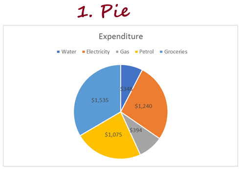
• Pie
  The other 2D pie is Normal Pie. It is used to show the contribution of each point to total value.
  
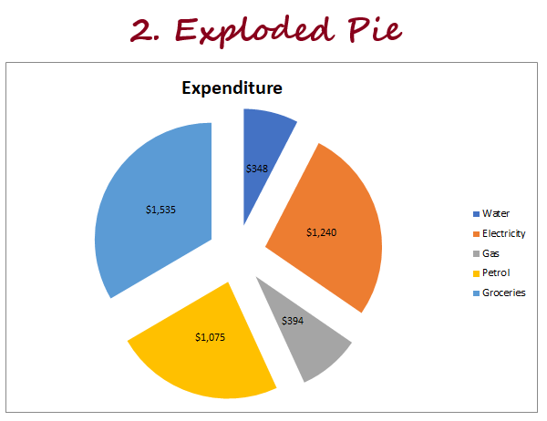
• Exploded Pie
  Exploded Pie shows the contribution of each value to total value while emphasizing individual data values. You can also ‘explode’ a normal pie by first clicking on the pie and then selecting a slice and then dragging it away from the center.
  
• PIE of PIE Chart
  Pie of Pie chart is used to extract some values from the main pie and combine them to the second pie. Using this chart you can make small percentages more readable or can emphasize more values.
  
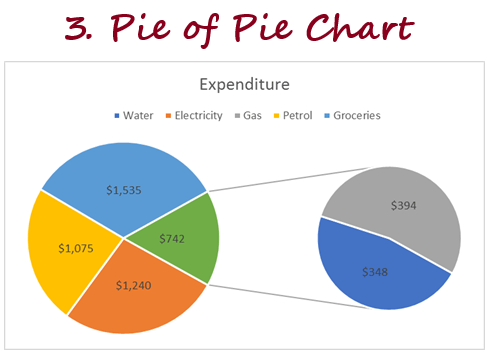
  As you can see in the above example, we have created two different pie charts where the first one is our original Pie chart, and the second pie chart represents the subset of the main pie chart.
• Bar of PIE Chart
  Bar of Pie Chart is used to extract some values from the main pie and combine them into a stacked bar. Using this chart you can make small percentages more readable or can emphasize more values.
  
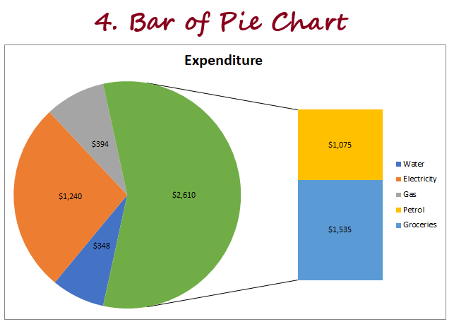
  As you can see in the example, the Bar of Pie chart is similar to Pie of the pie chart, but with the only difference that instead of a sub pie, a sub bar will be created.

Eureka! We have successfully covered all the different types of 2D charts, and now we will move to 3D Pie charts.

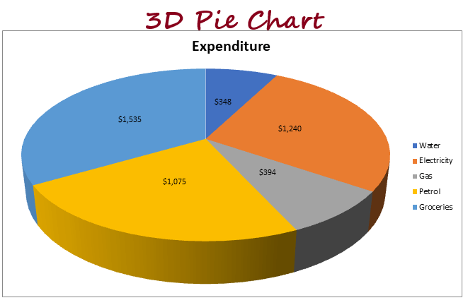
2. 3D PIE Chart

There is not much of a difference between 2D and 3D pie charts. Both are almost the same with a visual difference. That’s because 3D charts have depth as well in addition to length and breadth (where 2D charts only have length and breadth).

Steps to Create a Pie Chart

Follow the below steps to quickly create a pie chart in Excel:

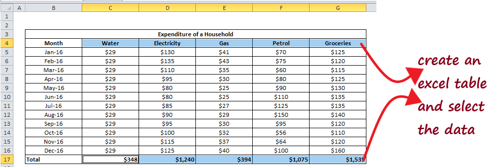
1. Create an Excel table and select the data for which you want to create a pie chart.
   
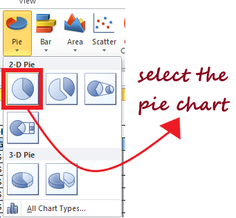
2. Go to the Insert tab in the toolbar at the top of the screen. In the Charts group, click on the Pie Chart option.
   
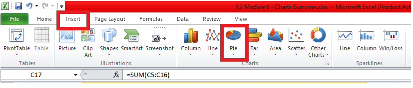
3. It will throw a drop down menu, select the appropriate chart and it will get incorporated in your Excel spreadsheet. In our case as you can see in the below image we have chosen the first pie chart (called Pie) in the 2-D Pie section.
   
4. Excel will create the pie chart with proper divisions where each division represents the 5 different types of expenditures.
   

You can beautify and format it further by writing the correct chart title, axis titles, changing the colours of the slices, adding legends, changing axis and trying different ways to format the chart.

Things to Remember

1. You cannot use negative data points in Pie charts as they treat them the same as positive values and do not show any difference in the chart. Therefore, it dilutes the output causing unnecessary confusion.
2. Pie charts work best with fewer data points. It is also advisable only to use 7 or fewer chart slices. Adding more than 7 divisions will make the chart look cluttered and impact the visibility.
3. It is always advised to use different colours for each chart division as it helps the users to distinguish between different pie slices quickly.
4. PIE charts are commonly used to represent simple and ordinal data points.