

[lwptoc]
Sheet Formatting
In this lesson you can learn everything about formatting in Excel.
Formatting can be done in Excel in two ways:
Using one of the prepared style (tables, charts, etc.) or
Formatting separated elements.
Using the prepared style is comfortable for novice users who use the standard tables or charts. Persons who wish to have full control over the appearance of a worksheet, or documents prepared by them do not fit within the imposed format, choose self-formatting. Using styles is discussed at the end of this lesson.
Method 1 Formatting step by step
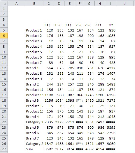
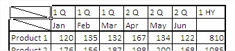
Suppose we were asked to prepare a table of data in the system as below. We managed to collect relevant data and paste them into the table. The following table, however, has many drawbacks.
Let’s take a look what to do next.
You’ve just opened a new workbook in Excel.
Change width of columns and rows
We’ll start with the fact that all data and descriptions of the categories are shown. At this time, the data in the cells ‘I23’ and ‘I32’ do not fit in the current column width and have been replaced by Excel on the symbols # # #.Similarly. The descriptions in cells B10 and B32 are also not shown in its entirety. To expand a column will be most convenient to double-click on the dash between the columns. You can also click and drag left button to expand the column width to the desired size.
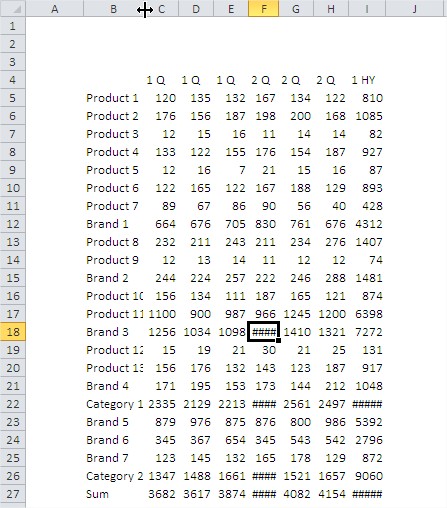
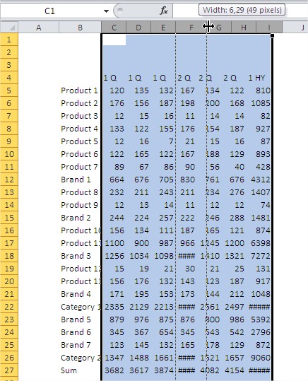
For columns of equal width, select all of which are to be aligned and drag the width of any of them to the desired size.
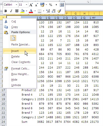
Insert / Delete rows
The next step is the removal of three rows at the beginning of the table. To do this, select the first three rows of the worksheet, select the rows by clicking on the symbol ‘1 ‘and holding the left mouse button pressed drag the selection to three-line, where he let go hold down the left key. Once selected, click on one of the signs of rows (1.2 or 3) and with the right mouse button menu that will select the Delete option.
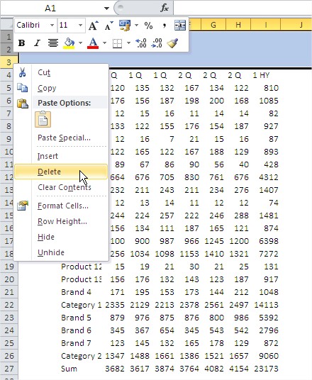
Will be deleted as many items as you previously selected. In the same way, you can insert rows or columns (the command ‘Insert’). Let’s insert now one line before the table.
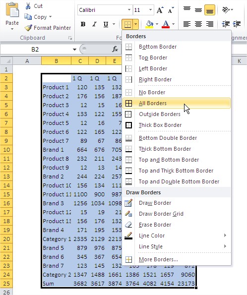
Borders
When you insert a row at the beginning of the worksheet, you activate the entire table and clicked on the icon bar arrow next to ‘Borders’ Proposes to select ‘All edges’ (marked in the figure below) for the entire table. Then ‘thick edge of the field’ (the two commands below) to make a bold border.
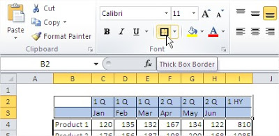
Now you can select only the cells of the column headers and select them again in bold borders. You will do the same for the row. You do not need every time to develop menu Borders, the last of the commands will be executed when you click the selected icons in the figure below.
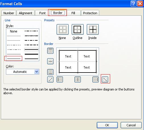
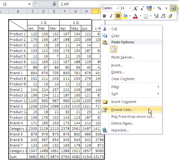
Border icons provide basic and most frequently used border, but you wanted to take advantage of dual or diagonal lines dividing cells should click with right mouse button on a selected cell, or the previously selected area and a menu that shows up, select ‘Format Cells …’.
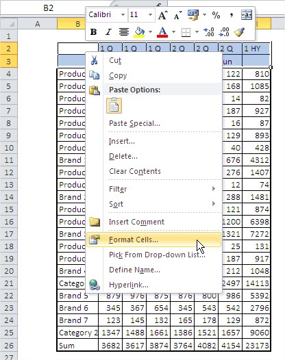
Window appears and ‘Format Cells’ on the ‘border’ you have all the formatting options that Excel offers. First, choose what format the line we are interested in the ‘Style’ and then click on the right side to indicate where the line is to be found, choose a diagonal line marked red square.
Merge cells
Another operation will merge cells. In cells B2 and B3 are diagonal lines that do not look good.
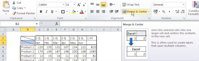
Select the cells you want to merge and click the icon for “Merge and center.”
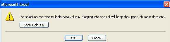
A message appears that symbols of 2 cells 1Q with a gray background in the picture above will be deleted. Click OK.
After the cells merged, I2 and I3, we find that we would prefer to headline 1HY (first half of the year) was displayed at half height of the new merged cell. Click the right mouse button and choose the command ‘Format Cells …’.
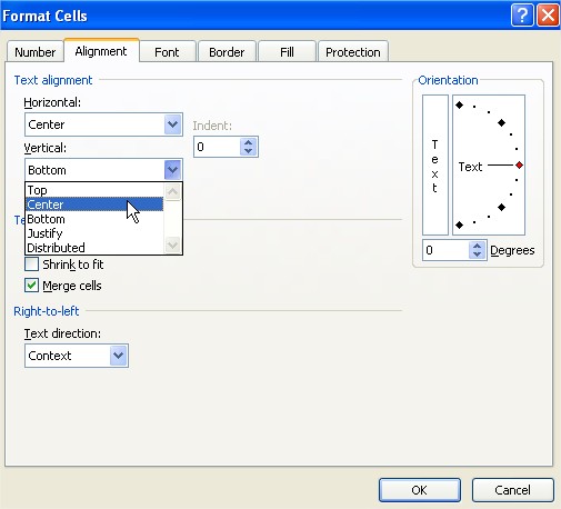
In the ‘Format Cells’ on the ‘Alignment’ choose ‘agent’ in the menu ‘Vertical’.
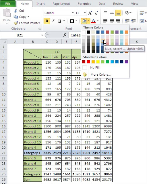
Change cell background color
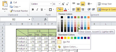
Change the background color of a cell or cell area, is to select the cell / area, click on the arrow next to ‘fill color’ (shown in the figure below) and select the desired color.
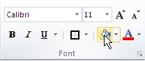
If we again color the cells of the same color, we need not choose it again, he was remembered, and simply click on the icon ‘fill color’.
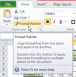
Format Painter
If you have some kind of format the cell, column or row and want you to another cell or area have the same format, instead of repeating all the operations from scratch, you better use the Format Painter. format line 21, as shown below. For bold, click the icon for B. The next step will be to change the color of cells, so that the aggregated data for the categories stand out.
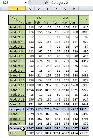
Just want to format several other rows. Of course, not every time we repeat the same steps, but we will use the ‘Format Painter’. Select the area of ‘pattern’, ie the line of 21st Click the Format Painter icon (paintbrush).
Click in cell B25 and the entire row of the table takes the appropriate format.
You can copy formatting from one cell immediately adjacent to a larger number of cells and copy the formatting of a larger area to area. It is not possible to copy the format once again after the first copy, Excel, ‘forget’ model after its first use and the operation must be repeated. Another way to format a number of areas so it is the simultaneous selection before formatting. To select multiple areas at once is enough while selecting with the mouse hold down the Ctrl button.
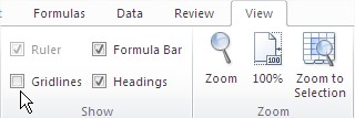
Gridlines
Reports and tables usually look better if you disable the grid lines. To enable or disable Gridlines tab to select the ‘Page Layout’, ‘Gridlines’, ‘View’.
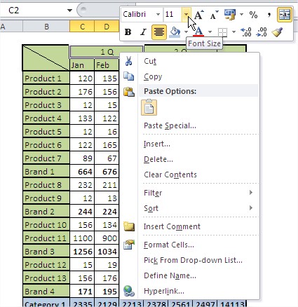
Change font size
To change the font in a cell or cell area is easiest to select an area for which you want to do it, then select the correct size from the drop-down box located in the icons (shown below). I recommend using the icons next to the first of which enlarges the font and the other decreases.
Hide / unhide rows and columns
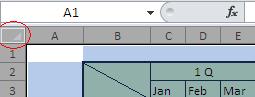
Hiding rows or columns is to select them To select all rows at once and all the columns simply click the left mouse button on the rectangle marked in the figure below a red circle.
To then discover all the rows, click the right mouse button on any determination of the line (below the red circle) and the menu that will select, Discover ‘, do the same for columns give us the assurance that all cells in the spreadsheet are visible.
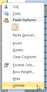
The data in hidden cells remain unchanged and are still employed by the formula. NOTE: The charts in Excel do not use the data in hidden cells.
Avoiding the destruction of formatting
The basic principle should be to format the cell deposition at the end of our work, once we sure that the system will be our report. If we do this earlier, pasting, copying and other operations, they can spoil our format and we have to do it again. Often, however, after the formatting changes are inevitable.
Style
Excel developers have prepared several formats, which can be used in preparing documents in Excel. Their biggest advantage is that inexperienced users can quickly get excel sheet professional. Styles work correctly only for simple tables or other objects.
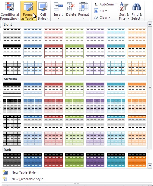
Method 2 Formatting as a Table
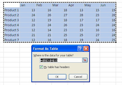
On the worksheet ‘Format 2’ is a table of data. It contains only one row of column headers and does not have catfish, so it can be formatted as a table. Set the active cell in any table cell and from your ‘Home’ to choose ‘Format as Table’, then choose the color model that suits us.
A window will appear, in which we are asked to confirm whether the area of the table was properly recognized. Click OK.
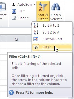
The table is formatted according to the selected model. If it does not suit us, that header cells contain symbols of the filter can be disabled by selecting ‘Sort & Filter’ and then click ‘Filter’.
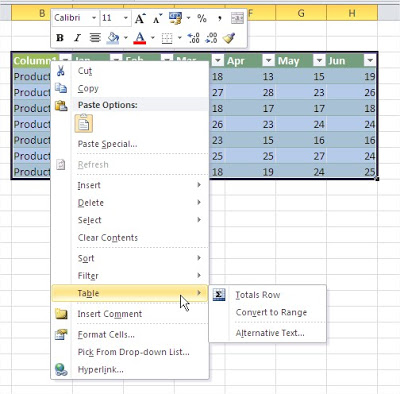
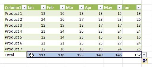
When you click the right mouse button on the table, we can add a row sum, as is shown below.
Sum which will be introduced only for June, copy to the other months.
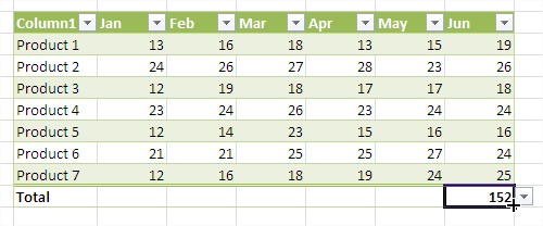
Exercise can be considered completed.
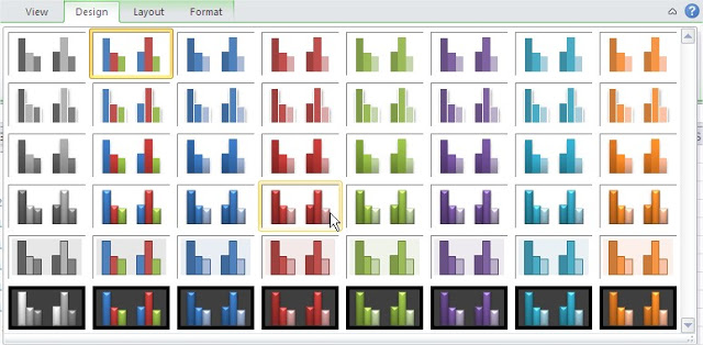
This way you can not format the table of Example 1, because it contains two rows of column headers. Example 3 There is a column chart. When you select it (by clicking on it with the left mouse button), command tabs appear: ‘Design’, ‘system’ and ‘Format’. On the ‘Design’ styles will find a chart, click on the arrow marked below the red square to view all available styles.
This way you can not format the table of Example 1, because it contains two rows of column headers. Example 3 There is a column chart. When you select it (by clicking on it with the left mouse button), command tabs appear: ‘Design’, ‘system’ and ‘Format’. On the ‘Design’ styles will find a chart, click on the arrow marked below the red square to view all available styles.
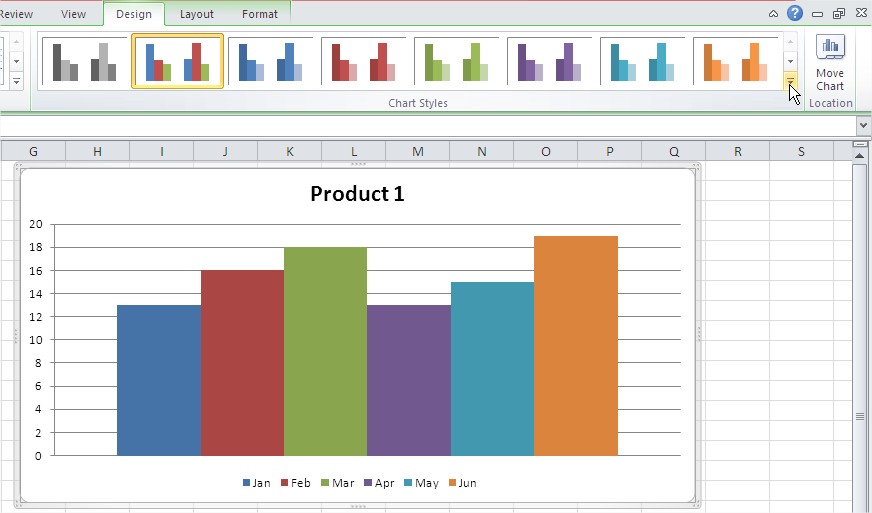
Choose the style that suits us and click on it.
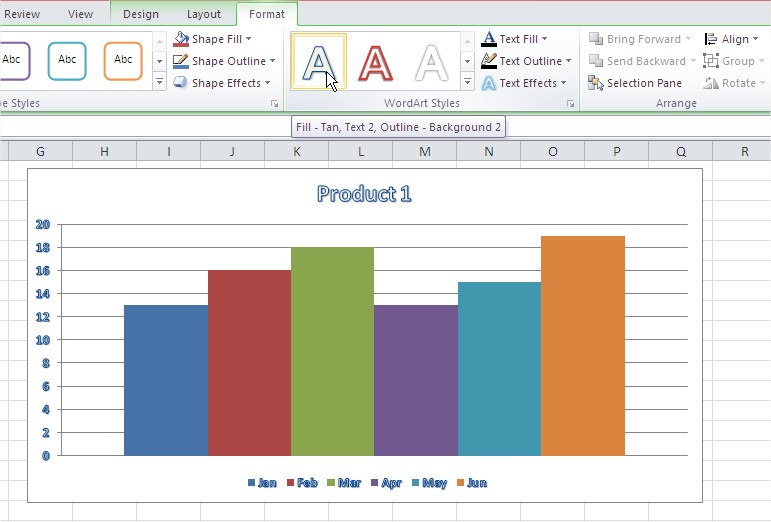
After changing chart style, even change the font style of his title. Select the title by clicking on it and the cards ‘Format’ select one of the WordArt styles.
Formatting Excel spreadsheets to be sure the look was tailored to the tasks to be satisfied by a given sheet. A common mistake beginners is the use of sophisticated style to impress the recipient, but unfortunately it does only feel the lack of professional approach.
Further reading:
Status Bar
Keyboard shortcuts
Display Cells Containing Formulas


