

Unhide Shortcut in Excel
MS Excel is currently the most popular spreadsheet software for data analysis and many other business-related tasks. Excel can easily store vast amounts of data. There may be cases when we need to hide some data that is unimportant to show others. In such cases, we hide the data using the Hide feature in Excel. However, we might later need to unhide it. For such a case, the unhide feature is the solution.

In this article, we discuss some quick shortcuts to unhide the hidden data in excel. The article explains all the steps and the relevant examples.
What is Unhide feature in Excel for Rows and Columns?
The unhide feature helps users to display the hidden data within the sheet. It is nothing but the opposite process of the hide feature in Excel. The unhide feature can help unhide the desired row(s)/ column(s) easily.
For example, suppose we have an Excel sheet where some rows have data that we don’t want to display to another person. However, we need to show a person the summarized analysis or the stored data results in the sheet. In such a case, we typically hide certain rows or columns. Later, we may again need to see the hidden data for further work or corrections. Thus, it becomes essential to unhide the data for facilitating a complete data view.
Unhide Rows and Columns using Keyboard Shortcut
Excel supports many keyboard shortcuts for performing various essential operations. Using the keyboard shortcuts reduces the overall working time and makes the process a lot easier and smoother. Since it is the fastest way to quickly perform most operations in Excel, we must know the shortcut keys to unhide rows and columns in Excel.
Since row and column are two different components of Excel, and they both act differently, we have different shortcut keys to unhide rows and columns:
For Rows
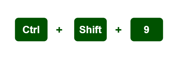
A keyboard shortcut to unhide a row in MS Excel is “Ctrl + Shift + 9” without quotes. We must perform the below steps to unhide a row in Excel with ease:
- First, we need to select one row on either side of the hidden row.
- After selecting the rows within the range, we must use the keyboard shortcut.
- As soon as we use the shortcut, all the hidden rows within the range will be unhidden from the visible screen.
For Columns
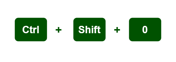
The keyboard shortcut to unhide a column in Excel is “Ctrl + Shift + 0” without quotes. We must perform the below steps to unhide a column in Excel with ease:
- First, we need to select one column on either side of the hidden column.
- After selecting the columns within the range, we must use the keyboard shortcut.
- As soon as we use the shortcut, all the hidden columns within the range will be unhidden from the visible screen.
Note: To use keyboard shortcuts for unhide feature in Excel, we must only use the numeric keys from the keyboard numbers instead of the number pad. Furthermore, the keyboard shortcuts may not work in Excel 2010 and earlier.
In Excel 2010 and earlier, we can use “Ctrl + Shift + (“ to unhide rows and “Ctrl + Shift + )” to unhide columns. Here, we don’t need to use the quotes while using the corresponding shortcuts. These legacy keyboard shortcuts also work in later versions of Excel.
The keyboard shortcuts to unhide the rows/ column in Excel do not always work for each machine, especially for systems based on Windows 8, Windows 10, and later versions. It is because Windows 8 and Windows 10 typically use the shortcut combination ‘Ctrl + Shift’ for Regional/ Language settings for changing keyboard layouts. Thus, the shortcut messes up with the system defaults. Therefore, to fix this issue, we must change the default keyboard layout shortcut with another key combination using the following steps:
- First, we need to launch the Control Panel and select ‘Change keyboards or other input methods’.
- Next, we will see a ‘Region and Language’ dialogue box where we must click the ‘Change Keyboard’ option under the ‘Keyboard and Language’ tab.
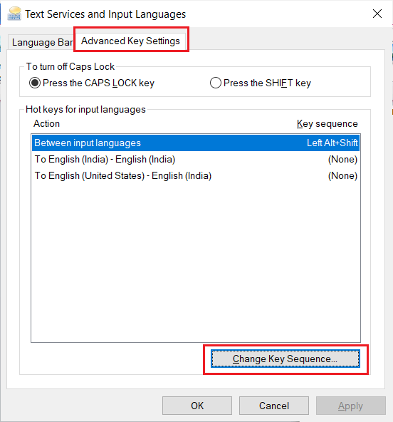
- On the next window, ‘Text Services and Input Languages’, we need to click the ‘Change Key Sequence’ option under the ‘Advance Key Settings’ tab.

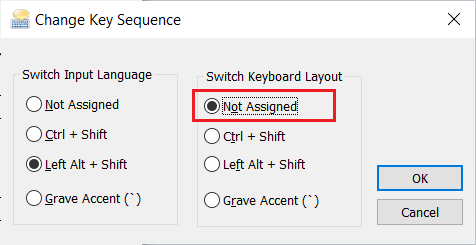
- Now, we need to navigate ‘Switch Keyboard Layout’ and set the radio button to an option ‘Not Assigned’ to disable the corresponding feature. However, if we need to use that feature, we can use other options to make this work. After making the desired changes, we need to click the OK button.
By doing this, we disable the shortcut ‘Ctrl + Shift’ for Regional/ Language settings for changing keyboard layouts. Thus, it starts working for the unhide feature in Excel.
Example
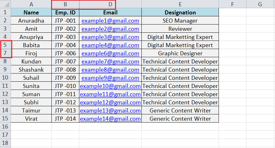
Consider the following Excel sheet with some employees’ data. We have a hidden row (i.e., 6th row) and a column (i.e., column C) in the following sheet. We need to unhide the corresponding row and column to make the data visible on the screen using the keyboard shortcut.
We need to perform the following steps to unhide the desired row and column in an example sheet:
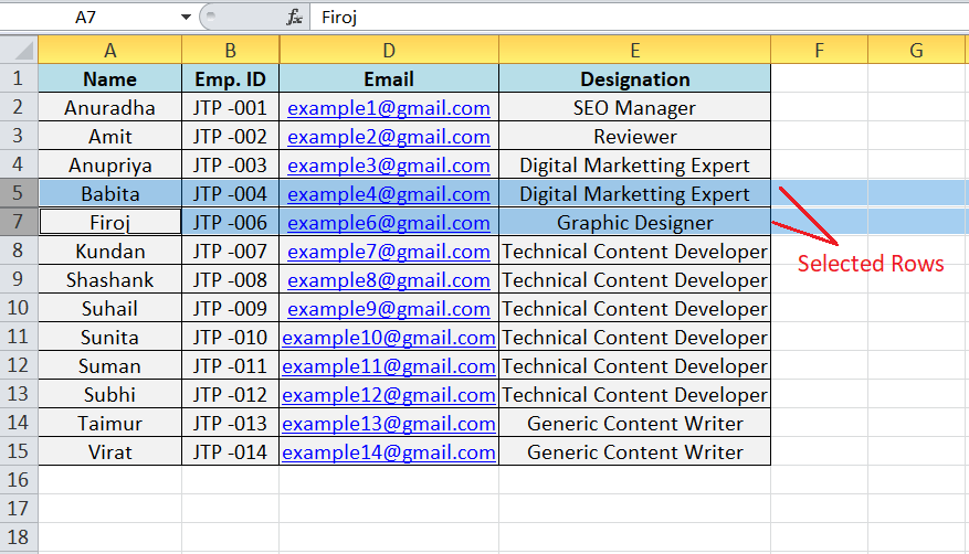
- First, we need to select the specific row on either side of the hidden row. This means we must select a row above and below the hidden row. In our case, the 6th row is hidden. Thus, we must select the row 5th and the row 7th.
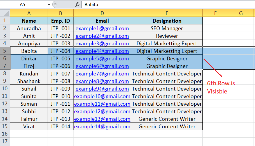
- After selecting one row on either side of the hidden row, we must use the shortcut ‘Ctrl + Shift + 9’ to unhide the desired row, i.e. 6th row. After we unhide the row, we can see it visible on the screen with its data, as shown in the following image:
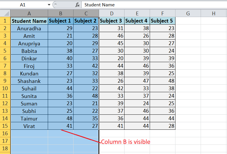
- After we unhide the desired row, we follow the same procedure for the column. This means we must first select one column on either side of the hidden column and then use the shortcut ‘Ctrl + Shift + 0’. Specifically, we select column B & column D and then press the shortcut key.
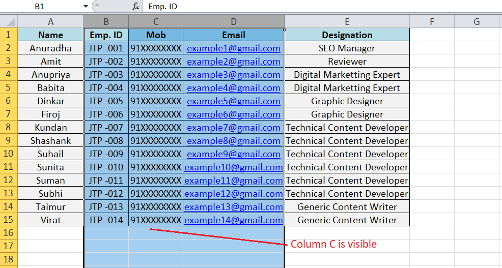
The data is completely visible on the screen as the desired row and column are both visible.
That is how we can use the Excel Unhide keyboard shortcut and unhide a desired row or column.
Unhide Rows and Columns using the Context Menu Shortcut
The simplest method to unhide the desired row or column in Excel involves using the context menu. The context menu is usually accessed by pressing right-click button on the mouse while the cursor is present on the corresponding row header or column header. This menu displays some essential options along with the Unhide feature. However, we must select the entire row or column; otherwise, the context menu will not appear.
For Rows
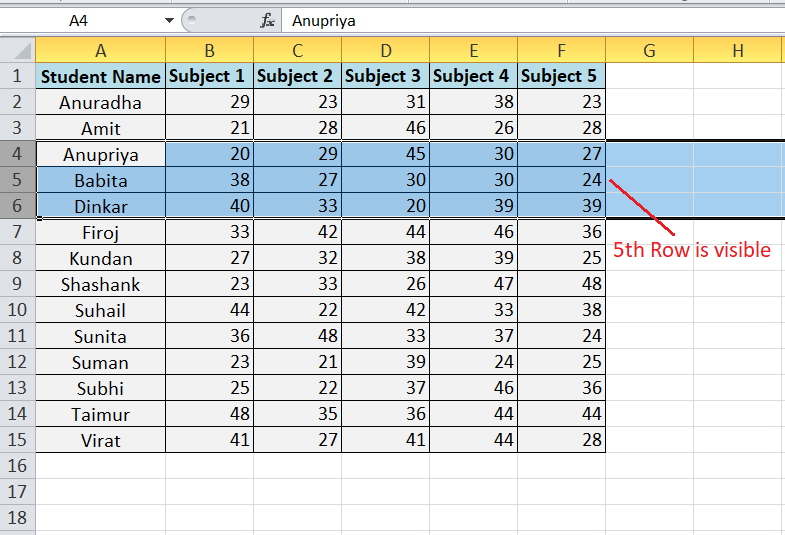
To unhide a row, we need to press the right-click button on the specific row header. However, we must first select one row on either side of the hidden row. For example, consider the following Excel sheet where we need to unhide the 5th row.
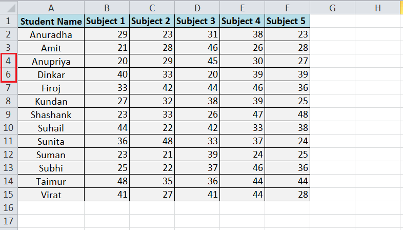
- First, we must select one row above the hidden row and one row below the hidden row. This means we select the rows 4th and 6th entirely.
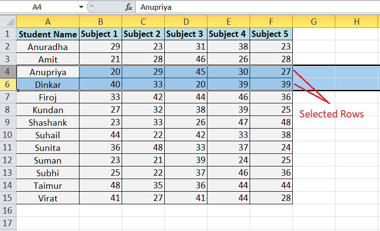
- Next, we need to move the cursor on the row header of any rows 4th or 6th and press the right-click button using the mouse.
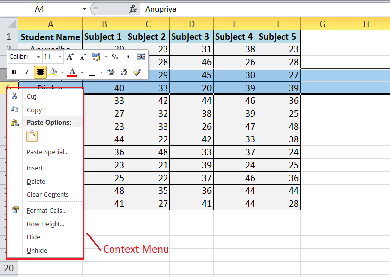
- Lastly, we must select the Unhide option from the list of the context menu.
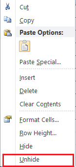
- As soon as we select the Unhide option from the context menu, the hidden row and the data become visible on the screen, as shown below:
For Columns
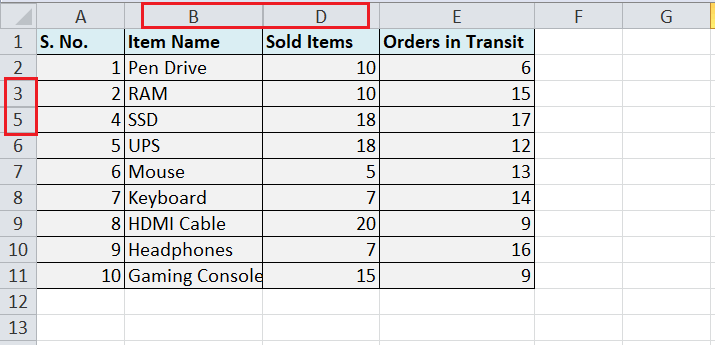
To unhide a column, we need to press the right-click button on the specific column header. Like the rows, we must first select one column on either side of the hidden column. For example, consider the following Excel sheet where we need to unhide column B.
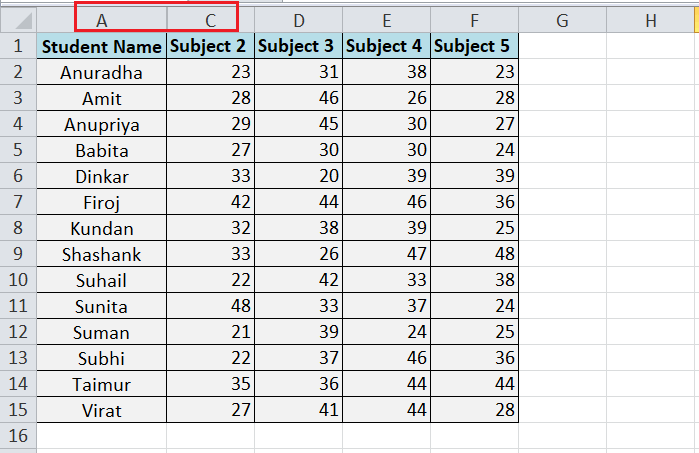
- First, we must select one column left to the hidden column and one right to the hidden column. This means we select columns A and C entirely.
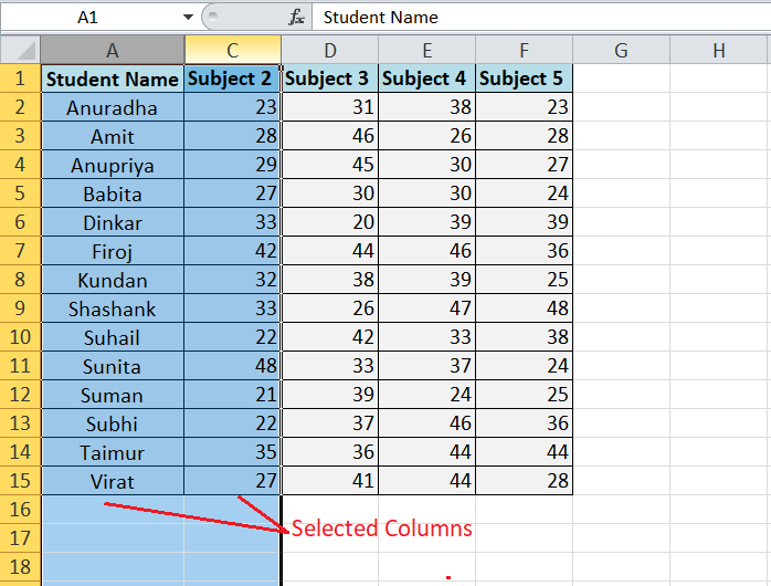
- Next, we need to move the cursor on the column header of any corresponding columns (column A or column C) and press the right-click button using the mouse.
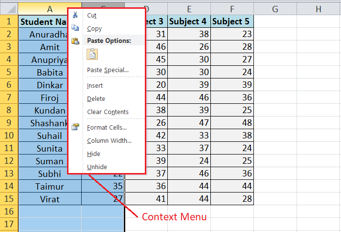
- Lastly, we must select the Unhide option from the list of the context menu.
- As soon as we select the Unhide option from the context menu, the hidden column and the data become visible on the screen, as shown below:
Unhide Rows and Columns using the Ribbon and its Shortcuts
Another essential method to unhide a desired row and column involves using a specific shortcut from the ribbon. This is a usual method to unhide a row or column. According to this method, the process is almost the same for both the row and column.
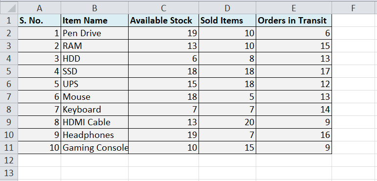
Suppose we have the following excel sheet in which we need to unhide the 4th row and column C.
Let us discuss the steps:
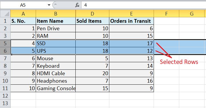
- First, we need to select the specific rows or columns on both sides (left & right for a column, above & below for a row) of the hidden row/ column. To select the rows above and below the 4th row (hidden row), we must click the row header of any corresponding rows and drag it to the other one.
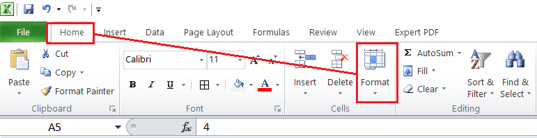
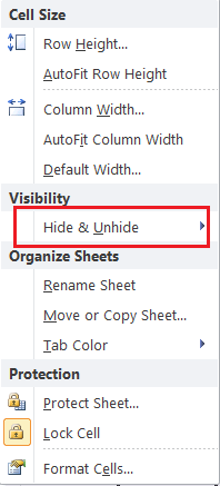
- Next, we need to navigate the Home tab and click on the Format option, as shown in the following image:
- After that, we need to choose the option ‘Hide & Unhide’ under the Visibility tab.
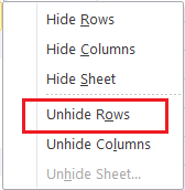
- Lastly, we choose a desired option from the list. To unhide a row, we must click the option ‘Unhide Rows’. Similarly, to unhide a column, we must click the option ‘Unhide Columns’. Since we need to unhide the 4th row, we select the option ‘Unhide Rows’.
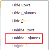
- Similarly, we select column B and column D and then select the option ‘Unhide Columns’ from the list to unhide column C.
After we unhide the desired row and column, the corresponding data becomes visible.
Despite clicking the shortcuts from the ribbon manually with the mouse, we can also use the sequence of keyboard keys to access the same. We need to press the following keys to perform the respective actions:
| Keyboard Keys | Action |
|---|---|
| Alt + H + O + U + O | Unhide Rows |
| Alt + H + O + U + L | Unhide Columns |
However, we must select one row/ column on either side of the hidden row/ column before using the keyboard keys mentioned in the above table.
Unhide Rows and Columns using the Double-Click Shortcut
Using the mouse double-clicks is another typical method to unhide a row or column quickly. For this, we must perform the following steps:
- First, we need to select one row/ column on either side of the hidden row/column, respectively.
- Next, we need to double-click on the double-line icon in between the row or column headers/labels, as shown below:
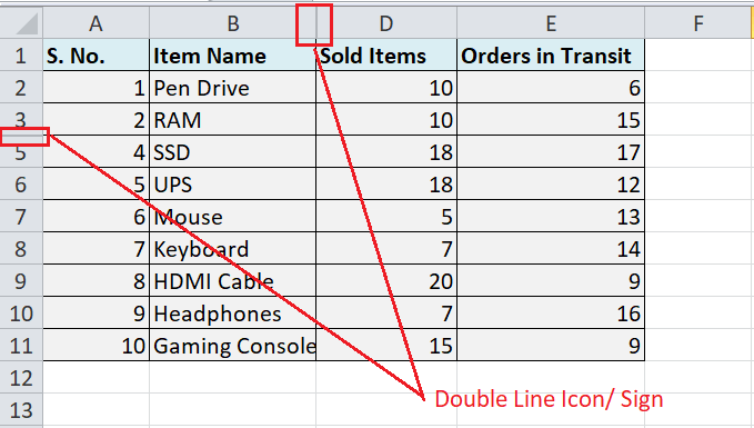
Doing this will instantly unhide the corresponding row/ column.
How to unhide multiple rows/ columns in Excel?
When multiple rows or columns are hidden within the sheet, we can select the connected rows or columns of both sides to the hidden row/ column and use any of the methods discussed above. To select multiple rows in a sheet, we must press and hold the Ctrl key and click the desired rows/ columns headers using the mouse.
For instance, we have the following sheet with rows 3rd and 7th hidden. To unhide them, we need to select the rows from both sides of the hidden rows. Thus, we select the 2nd & 4th rows and then the 6th & 8th rows.
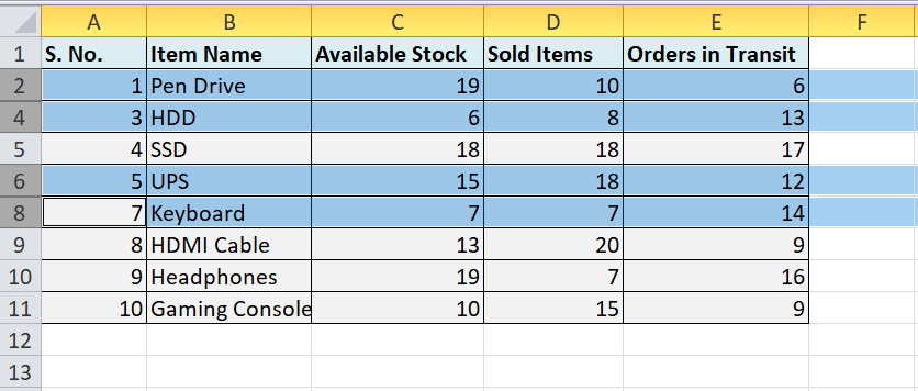
Next, we navigate to the format option under the Home tab and choose the unhide rows from the drop-down. Similarly, we can unhide the multiple columns.
How to unhide all rows and columns in an Excel sheet at once?
When there are several hidden rows and columns within an Excel sheet, it becomes a tedious task to select many rows and columns and use the unhide shortcut. Therefore, we must perform the following steps and then the unhide shortcuts:
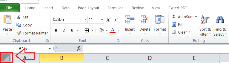
- We need to select the entire sheet at once instead of selecting specific rows or columns. For this, we can either use the keyboard shortcut ‘Ctrl + A’ or click the triangle icon left to the column A label.
Once the entire sheet is selected, we need to use any of the unhide shortcuts discussed above. We can use Alt + H + O + U + O to unhide rows and Alt + H + O + U + L to unhide columns. However, we must press one key at a time while using the specified shortcut keys.


