Borders and Shades in Excel

MS Excel is powerful spreadsheet software that helps users store data across multiple worksheets. Each worksheet contains several cells formed by the intersection of rows and columns. By default, the Excel cells have no borders and use white shades. However, borders or shades can help make data easy to read or highlight when we have a large data set.

Apart from this, it becomes too complex to read when we take prints of worksheet data without borders. Excel allows us to add a border and color shades to one or more desired cells within the worksheet.

Borders and Shades (Shading)

In Excel, borders refer to a line drawn across any or all of four sides of a cell in a worksheet. When adding a border to one or more cells, we can choose specific sides to include or exclude. Moreover, we can also manually draw borders for custom or desired sides of cells. For example, we can add (or draw) borders to the top and bottom of the cell and leave the other sides open.

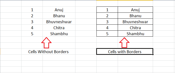
Furthermore, shading refers to an artistic design or color used as the background of a cell in a worksheet. When adding shading (background color) to one or more cells, we can choose one of the pre-defined colors set for a specific cell. Additionally, we can also choose a custom color for the desired cell.

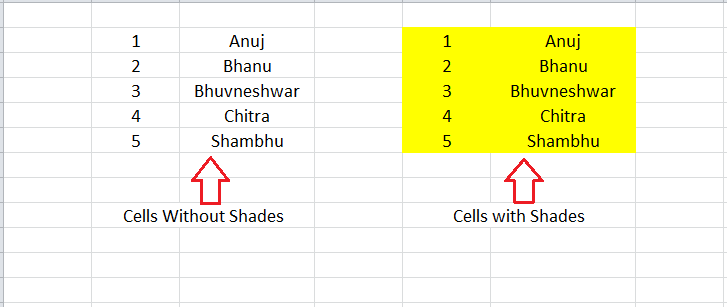
Let us now discuss how we can add/remove color or shading from a cell within an Excel worksheet:

Applying Borders in Excel

Creating a border is one of the easiest things to do in Excel. Although there are several methods, this is usually done using the following two methods:

Applying Borders from Ribbon

Excel Ribbon is the primary area for accessing most existing commands or tools. While creating a border in Excel, we can take advantage of the Excel ribbon and apply a border to the desired cell using the following steps:

• First, we need to select the effective Excel cells where we wish to insert borders. We can hold down the mouse’s left button and drag the selected shading from one cell to the others. Besides, while selecting non-adjacent (or non-contiguous) cells in Excel, we must click on individual cells while holding down the Ctrl key.
  
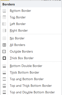
• After selecting the effective cell, we need to go to the Home tab on the ribbon and click on the drop-down icon next to Border, as shown in the following image:
  
• In the next window, Excel will display various pre-defined border styles. We must click on the desired border style to apply it.
  
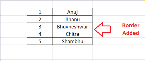
  After clicking on the desired border (for example, All Border) from the list, the same will be instantly inserted into the selected Excel cells.
  
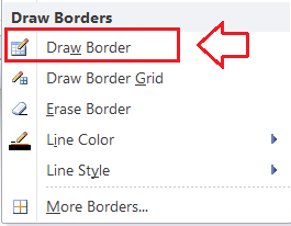
  Although there are many existing border options, sometimes, we may need to insert a border on specific sides of the cell manually. For example, suppose we need to add or insert a border on any cell’s left and right sides. We can manually draw borders using the Draw Border option from the drop-down list in such a case.
  
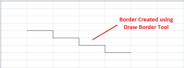
  After selecting the Draw Border option, our mouse cursor will convert into a pencil icon. We can click or drag on the desired grids to draw corresponding borders.
  
  Similarly, we can choose Line Color or Line Style options to color the desired borders or choose border-style like a single line, multi-line, etc.

Applying Borders from Format Cells dialogue box

Since adding a border is part of the Excel formatting tool, we can also apply a border using the Format Cells dialog box. We can perform the following steps to access the Format Cells dialog box and insert a border in the desired Excel cell:

• First, we need to select/ highlight the effective cells in the worksheet.
• Once the desired cells are selected, we need to launch the Format Cells dialogue box. The easiest option to access/open it is to use the keyboard shortcut ‘Ctrl + 1’. However, we must only press the key ‘1’ from the keyboard area, not the number keypad.
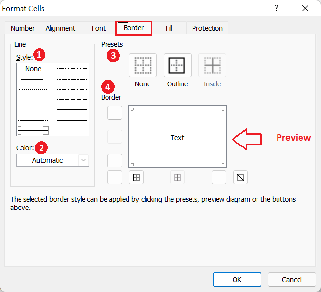
• In the Format Cells dialogue box, we need to click on the Border tab, as shown below:
  
  We can adjust the cell’s borders in multiple ways using different sections displayed in the above dialogue box:
  
  1. The Line Style section helps us select the desired design for the borders, such as single line border, dotted line border, double-line border, etc.
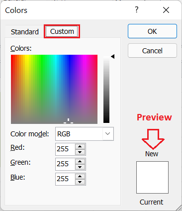
  2. The Color section or drop-down list under the Line category allows us to choose any desired color for the border. We can either choose the pre-defined colors or choose our custom color using the More Colors option.
  3. The Presets section helps us apply quick borders to the selected cells in the worksheet. Using Presets, we can select between None (no border), Outline (all sides borders), or Inside (borders in the connected sides of cells).
  4. The Border section helps us to choose different border styles. We can click on the displayed block to choose the top border, bottom border, left border, right border, diagonal border, etc. The preview section displays the border style as per the selected preference or settings in the dialogue box.

  After adjusting the settings for the borders, we must click the OK button to close the dialogue box and apply the changes in the worksheet.

Deleting Borders in Excel

To remove/delete border in the Excel worksheet, we can use any of the following methods:

• First, we need to select the cells from which we wish to remove borders. Next, we must go to Home > Border > No Border. This will remove the borders from selected cells. For selecting specific cells to remove the border, we can hold down the Ctrl key while clicking the corresponding cells.
• We can also delete borders using the Erase border tool. For this, we must go to Home > Border > Erase Border. This will convert the mouse cursor into the eraser icon, using which we can erase or delete the desired border in the worksheet.
• We can select the cells and go to Home > Clear > Clear Formatting. Although this method helps remove borders, it also removes other formattings like font color, background color, etc. Thus, this method may not be suitable in all conditions.

Applying Shades in Excel

Applying shades in Excel is as easy as creating borders. The following are the most commonly used methods for applying shades to an Excel cell or worksheet:

Applying Shades from Ribbon

The Ribbon provides quick access to Excel’s existing tools, and it is very easy to apply color shades from the Ribbon area. We can perform the following steps and use any desired shade or background color for the cell:

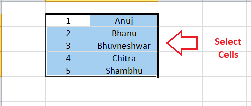
• First, we need to select the cells where we want to apply the shading.
  
• After selecting the desired cells, we must navigate the Home tab and click the drop-down icon next to the ‘Fill Color’ option, as shown below:
  
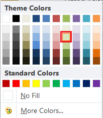
• Excel displays various colors under the Theme Colors and Standard Colors in the next window.
  
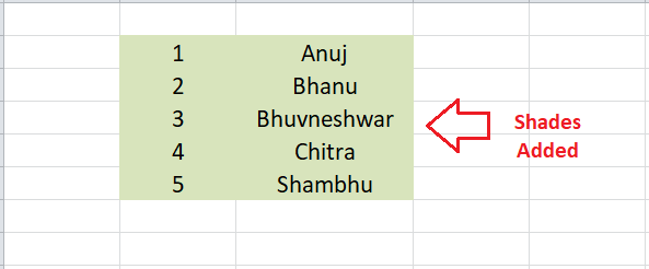
  We can click on any desired color, and the same will be immediately applied to the selected cell as a background color.
  
  If we don’t find the color we want, we can click on the ‘More Colors’ button from the window and choose any custom color accordingly.
  

Applying Shades from Format Cells dialogue box

We can use the Format Cells dialogue box to apply any desired color shades in Excel cells, like applying the border. We must select the cells, open the Format Cells dialogue box (Ctrl + 1), click the ‘Fill’ tab, and adjust the preference accordingly. The Fill tab contains the following sections or preference options:

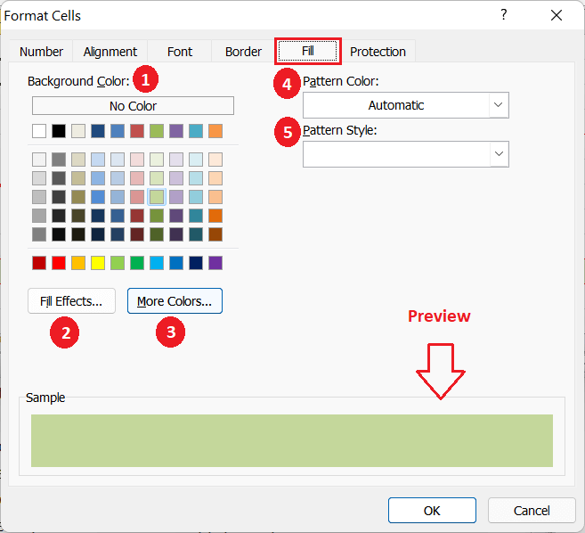
In the above dialogue box, we can apply or modify the color shades in various ways using different sections, such as:

1. This section displays a set of pre-defined colors. We can select the desired color by clicking on the respective block.
2. This section allows us to choose gradient-style shades. We can choose between one color or multi-color shades and gradient direction.
3. This section enables us to choose the color that is not available within the displayed blocks. Using this section (button), we can create any custom color we want.
4. This section allows us to choose the color for the pattern style we want to add along with the shades.
5. This section contains various pattern styles that can be applied along with the selected color shades. This includes dotted gray patterns, horizontal and vertical lines, diagonals, diagonal crosshatches, etc.

After adjusting the settings for the shades, we need to click on the OK button to close the dialogue box and apply the selected color shades to the desired cells within the worksheet.

Deleting Shades in Excel

When deleting or removing shades or background color of Excel cell(s), we can use any of the following methods:

• First, we need to select the cells from which we wish to remove shades. Next, we must go to Home > Fill > No Fill. This will immediately remove the color shades from the selected cells. To remove colors from the entire sheet, we can use the keyboard shortcut ‘Ctrl + A’ to select all cells in the sheet, then choose ‘No Fill’. To select specific cells, we can hold down the Ctrl key while clicking the corresponding cells.
• If we have just applied the shades in the cell, we can click Undo (Ctrl + Z) to remove them.
• We can select the cells and go to Home > Clear > Clear Formatting. Although this method helps remove color shading, it also removes other formattings like font color, border, etc. Thus, this method may not be suitable in all conditions.

Important Points to Remember

• After applying the border before printing the sheet, we must ensure that the border is printed using the Print Preview window.
• When adjusting the preference of color shades using the Format Cells dialog box, we cannot use the ‘Fill Effects’ and ‘Pattern Styles’ both with the color shades.
• We must make sure that the text within the cells is properly visible when applying the color shades.