Checkbox
Insert a Checkbox | Link a Checkbox | Create a Checklist | Dynamic Chart | Delete Checkboxes | Powerful Checkboxes
Inserting a checkbox in Excel is easy. For example, use checkboxes to create a checklist or a dynamic chart. You can also insert a check mark symbol.
Insert a Checkbox
To insert a checkbox, execute the following steps.
1. On the Developer tab, in the Controls group, click Insert.

2. Click Check Box in the Form Controls section.
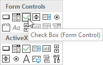
3. For example, draw a checkbox in cell B2.

4. To remove “Check Box 1”, right click the checkbox, click the text and delete it.

Link a Checkbox
To link a checkbox to a cell, execute the following steps.
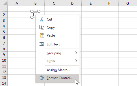
1. Right click the checkbox and click Format Control.
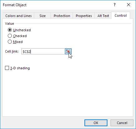
2. Link the checkbox to cell C2.
3. Test the checkbox.
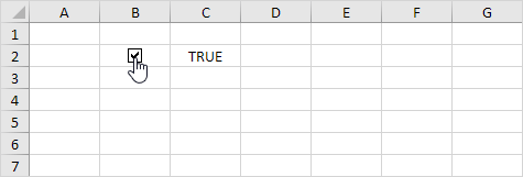
4. Hide column C.
5. For example, enter a simple IF function.
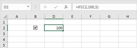
6. Uncheck the checkbox.
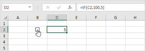
Note: read on for some cool examples.
Create a Checklist
To create a checklist, execute the following steps.
1. Draw a checkbox in cell B2.
2. Click on the lower right corner of cell B2 and drag it down to cell B11.
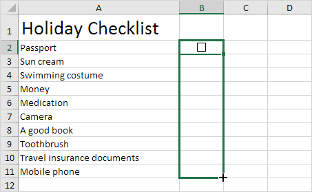
3. Right click the first checkbox and click Format Control.
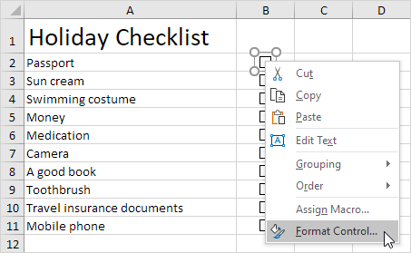
4. Link the checkbox to the cell next to it (cell C2).
5. Repeat step 4 for the other checkboxes.
6. Insert a COUNTIF function to count the number of items packed.
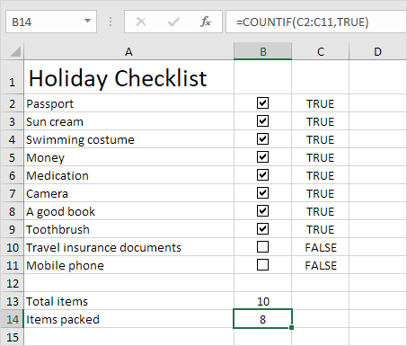
7. Hide column C.
8. Insert an IF function that determines if you’re good to go.
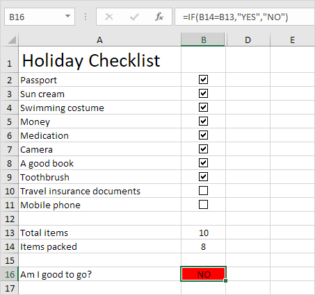
9. Click all the checkboxes.
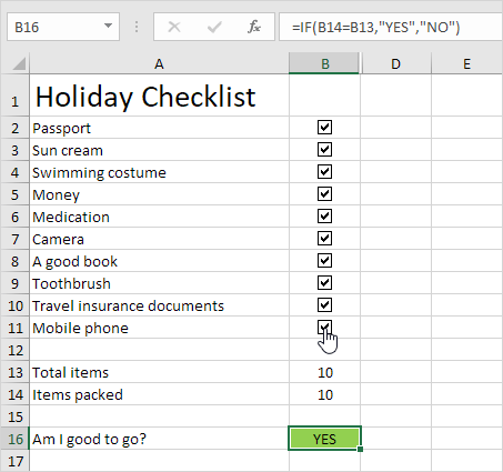
Note: we created a conditional formatting rule to automatically change the background color of cell B16. Try it yourself. Download the Excel file and test the checklist (second sheet).
Dynamic Chart
Let’s take a look at one more cool example that uses checkboxes. A dynamic chart.
1. For example, create a combination chart with two data series (Rainy Days and Profit).
2. Add two checkboxes.
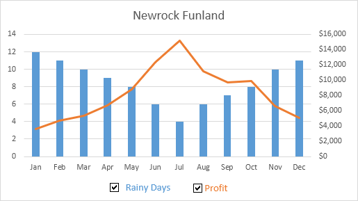
3. Right click the first checkbox and click Format Control. Link this checkbox to cell B15.
4. Right click the second checkbox and click Format Control. Link this checkbox to cell C15.
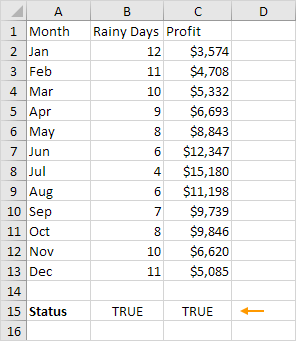
5. Uncheck the second checkbox. Cell C15 below changes to FALSE.
We’re now going to create two new data series.
6. Insert the IF function shown below. Use the fill handle to copy this formula down to cell F13.
7. Repeat this step for the new Profit data series.
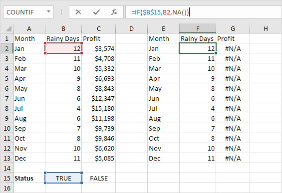
Explanation: if the checkbox is checked, the old and new data series are the same. If the checkbox is unchecked, the new data series changes to a range with #N/A errors.
8. Use the new data series to create the combination chart. To achieve this, select the chart, right click, and then click Select Data.
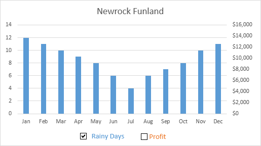
9. Uncheck the first checkbox and check the second checkbox.
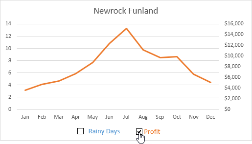
Note: try it yourself. Download the Excel file and test the dynamic chart (third sheet).
Delete Checkboxes
To delete multiple checkboxes, execute the following steps.
1. Hold down CTRL and use the left mouse button to select multiple checkboxes.
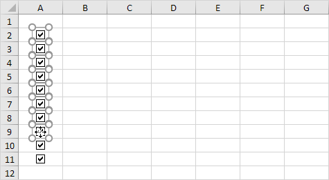
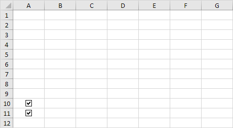
2. Press Delete.
Powerful Checkboxes
Finally, you can use VBA to create powerful checkboxes in Excel. Instead of inserting a Form control, simply insert an ActiveX control.
1. Insert a checkbox (ActiveX control).
2. At step 6, you can add your own code lines to automate all kinds of tasks. For example, add the following code lines to hide and unhide column F.
If CheckBox1.Value = True Then Columns(“F”).Hidden = True
If CheckBox1.Value = False Then Columns(“F”).Hidden = False


Note: maybe coding is one step too far for you at this stage, but it shows you one of the many other powerful features Excel has to offer.
Next Chapter: Workbook


