Circular reference in Excel
Generally, when you enter a formula in a cell to calculate some data, you provide the reference of other cells. But sometimes, you see when you enter the formula in an Excel sheet, it does not work. This happens when you use the resultant cell reference in the formula. Hence, you receive a warning message about the occurrence of circular reference.
You face this problem when your formula is trying to reference itself and the Excel feature called Iterative calculation might turn off. The formula may look like this –
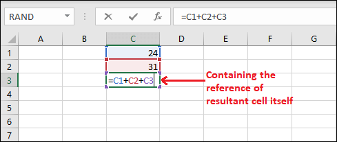
Here, C3 cell contains a formula that is performing the addition of three cells, including C3 cell inside formula for calculation. So, a circular reference refers to the formula that calculates its own reference.
Topics discussed in this chapter
Following topics we are discussing in this chapter –
- What is a circular reference?
- Example of circular reference
- What is iterative calculation?
- Enable or disable the iterative calculation
- Detect the circular reference
- How to remove circular reference?
- Why should avoid circular reference
- Types of circular reference
- How to find hidden circular reference
What is a circular reference?
A circular reference occurs when a formula refers to its own cell either directly or indirectly.
Direct circular reference
Direct circular reference occurs when a formula directly contains the reference of the resultant cell while performing any operation. In the following example, formula is written in C3 cell and contains its own cell (C3) reference in formula.
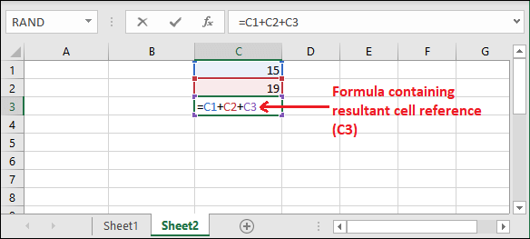
When you press the Enter key, a pop up will open and show you a warning message.

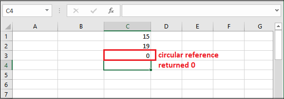
Click OK on this warning pop up window to close it and Excel will return 0.
Indirect circular reference
Indirect circular reference occurs when the different formulas are depending on each other cells data in circular manner. Below is an example for the indirect circular reference.
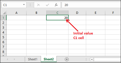
For this, we take a numeric value (20) in the C1 cell initially.
Step 1: Now, we have multiplied this value by 2 and stored it in the E5 cell. This way, E3 cell refers to the C1 cell.
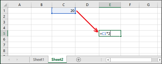
Step 2: Press Enter and get the calculated result in E5 cell.
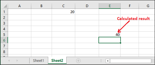
Step 3: Now, perform one more multiplication operation on E5 cell value by 2 and store it in the A5 cell. Here, A3 refers to the D3 cell.
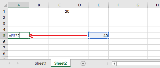
Step 4: Press Enter and get the calculated result in A5 cell.
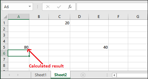
Till now, there is no circular reference in this sheet. Now, if we perform any operation on A5 cell data whose result will store in C1 cell, it will create an indirect circular reference.
Step 5: Remove the previous value from C1 cell and write the following formula in it.
=A5*2
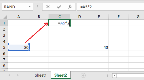
Step 6: Press the Enter key, it will generate an error message of circular reference.

Step 7: On this warning message, click the OK button. You will see it return 0 and also show you the created circular reference.
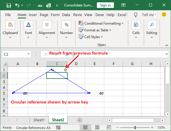
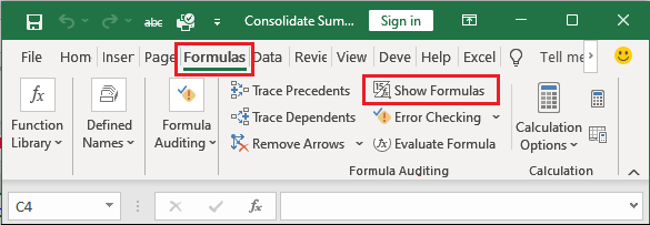
Step 8: Go to the Formula tab and click the Show Formula option inside the Formula Auditing group.
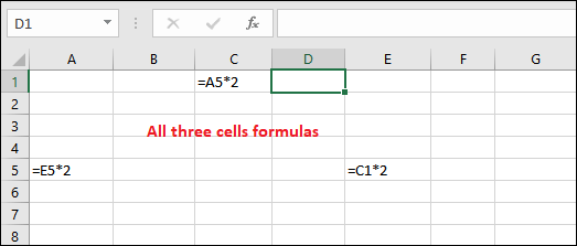
Step 9: It will enable the formulas used in all three cells. See in the below screenshot –
Step 10: Double-tap any of the cells; you will see the circular reference between all three cells.
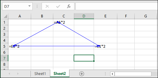
E3 cell refers to C1, C1 cell refers to A3 cell, and A3 cell refers to E3.
Example of circular reference
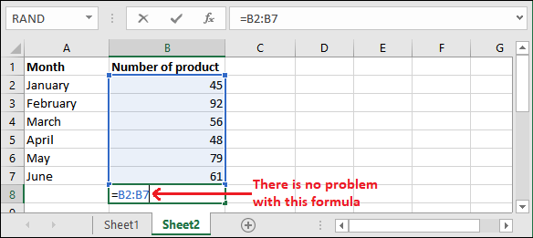
In this example below, we calculate the total sum of six months sell (cell B2:B7) and the result stored in B8 cell. There is no problem with this calculation, and it is calculated with no issue.
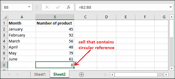
But in case if you accidently select the B8 cell reference that contains the result instead of B7. So, we are performing the calculation including resultant cell, like this –
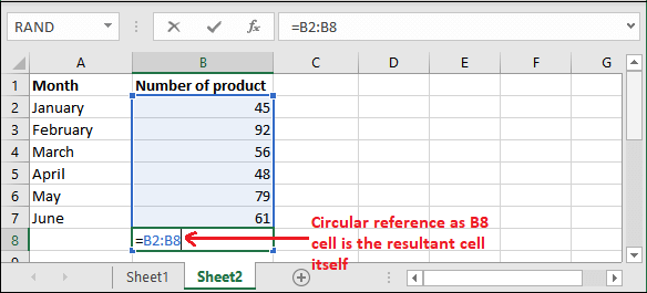
When you press the Enter key, it will give you a warning because this type of calculation is not possible. Excel warns the users for one or more circular references.

When you click the OK button on this warning pop up, this warning will close. You can also go for the Help option for more information.

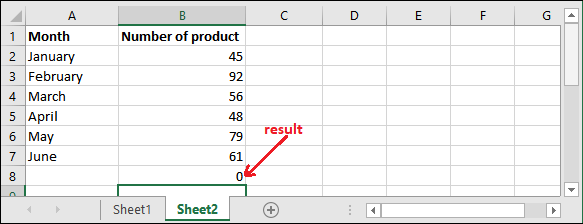
If you click OK, the value 0 will populate to the B8 cell which is selected to keep the result.
What is iterative calculation?
Iterative calculation allows the users to perform circular reference and recalculate the data using the resultant cell reference. Thus, you can allow circular reference in an Excel sheet.
A circular reference occurs when the formula includes the cell where your result will reside. It can be either directly or indirectly. Sometimes, you may require circular references. But when you accidently use circular reference, it returns 0 that is an unexpected result.
Excel offers an iterative calculation feature that allows the users to do repeated calculations until it meets a specific condition. You can enable the iterative calculation option in Excel to make the circular reference possible.
Enable or disable iterative calculations
In some cases, iterative calculation are repeated recalculations till when it meets a specific condition. If you want to use circular reference, you have to enable the Enable iterative calculation inside the Excel File menu. By default, this option (Enable iterative calculation) is turned off (unmarked).
Step 1: Click the File tab in Excel.
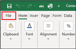
Step 2: On the left side of the Excel backspace, click the Options inside More….
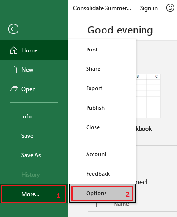
Step 3: Navigate to the Formulas tab in the left window and mark the Enable iterative calculation option here.
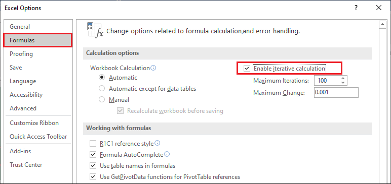
After that, click OK to save this change.

This way, you can enable the iterative calculations and once it is enabled, the user can control the maximum number of iterations as well as the maximum changes option. You should know what is the maximum iterations and maximum changes. So, here is detail description for them –
Maximum iterations – Maximum iterations refers how many times Excel will recalculate. You can define the maximum iterations. But if the number of iterations increases, calculation will take more time than before.
By default, the maximum number of iterations is 100. You can change it.
Maximum changes – Maximum changes defines maximum contracting between the values of iterative formulas. The result will be more accurate when smaller the number.
By default, the maximum number of iterations is 0.0001. You can also change it as well.
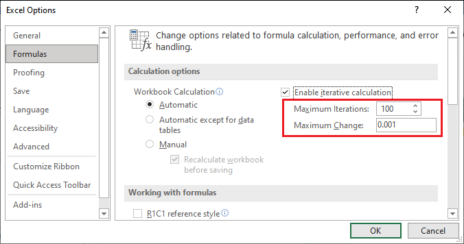
By default, maximum iterations are 100 and maximum changes are 0.0001. This means Excel will stop calculating after 100 iterations or after less than 0.0001 change.
Detect the circular reference
When you do not create worksheet by yourself and receive it from another, you do not is there any circular reference in it. So, to make sure there is no circular reference, you can manually detect the circular reference in file.
Method 1: From Error Checking
For this, follow the given steps below:
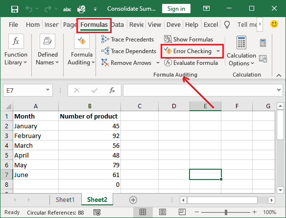
- Navigate to the Formula tab and click the Error Checking inside the Formula Auditing group.
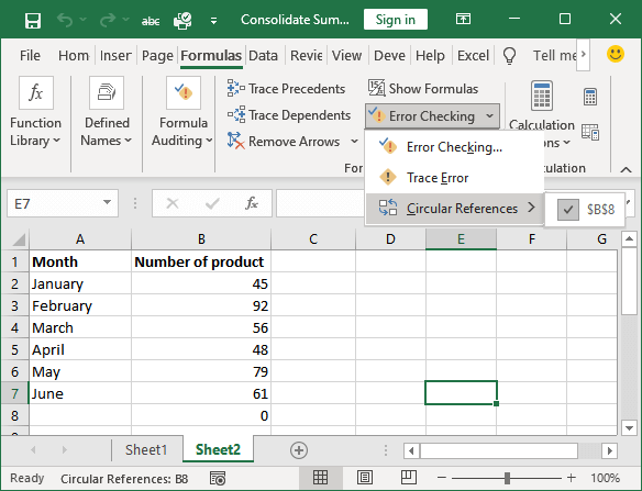
- Now, select Circular Reference from the list, i.e., Formula > Error Checking > Circular Reference.
Excel will show you the cell reference that contains a circular reference.
- Excel will exactly take you to that cell which contains circular reference in this Excel sheet.
Method 2: Directly from the status bar
Another way to detect the circular reference in an Excel sheet is to find it in Excel status bar. This one is the easiest way to find the circular reference in an Excel sheet.
If an Excel sheet contains circular reference on any cell, you will see the Circular Reference along with cell number written at the bottom (in the bottom left corner) of the Excel sheet.
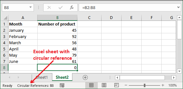
It also contains cell number where circular reference exists in your Excel sheet.
Tip: If the circular reference does not exist in the currently active sheet but not in another sheet of the same workbook, it will display “Circular Reference” with no cell number.
For example, Sheet2 contains a circular reference, but Sheet1 does not. So, the status bar for Sheet1 will be –
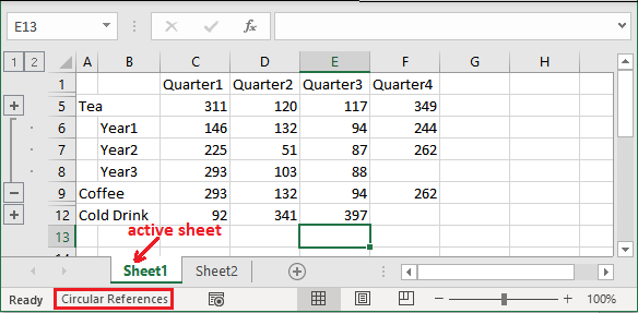
Ignore the sheet1 data.
How to remove circular reference?
Excel does not have any shortcut or predefined method to remove the circular reference from Excel sheet. You have to find each circular reference individually in the Excel sheet wherever it presents with the help of above steps. Then you need to remove them manually one by one. You can either remove the formula completely that creates circular reference or replace it with another formula.
Why should avoid circular reference?
The Excel user should avoid the usage of circular reference. It makes the Excel data more complex and can affect the performance too. Each time when you open the Excel sheet that contains the circular reference, a warning message will display to you like this –

But suppose you have allowed iterative calculation (by marking Enable iterative calculation). In that case, it will not display any warning message and even you cannot find the circular reference from the Error Checking inside the Formula tab. Besides this, circular reference may also lead to several other issues because of circular reference.
For example, if you select a cell with circular reference and accidently switch to the formula editing mode. Also, you have pressed Enter key without making any change in formula; it will return 0.
Note: Formula editing mode enables by pressing the F2 key or double-clicking the selected cell.
Circular reference has a high risk when you have a large data spreadsheet containing too many formulas. Once circular reference may cause to miscalculations.
Different types of circular references
You will find different types of circular references in Excel, such as –
- Unintended circular reference
- Intended circular reference
- Hidden circular reference
You will find most circular references as unintended. Excel automatically searches unintended types of instances for the users.
There are intended circular references as well. These types of circular references are usually made by experienced users and used to make iterative calculations.
One more type of circular reference, i.e., Hidden Circular reference. Hidden circular reference is hard to detect so they can be dangerous. The operation of this type of circular reference depends on another cell value.
How to find a hidden circular reference?
A hidden circular reference is hard to detect. So, we will describe the steps to find the hidden circular reference in an Excel sheet. Generally, when you open the Excel sheet that contains the circular reference, a warning message will display to you like this –

But if you have allowed circular reference by enabling the iterative calculation, then this warning message will not display. Even you cannot find the circular reference from the Error Checking option inside the Formula tab.


