

Data bars in Excel
Excel Data Bars is a really powerful feature for visualizing values in a range of cells. Based on some conditions, it can help you highlight the cells or data range in a worksheet. To make it more clearly visible, it is suggested to make the bars in the column wider.
The tutorial explains the basics of Excel Data Bars feature. You will discover how to add different data bars in Excel, how to edit the bars in any version of Excel.
What are Data bars?
Excel Data Bars feature are a type of conditional formatting options that combines Data and Bar Chart inside the cell. This tool indicates the percentage of selected value or where the selected data resides on the bars inside the cell.
Data bars in excel belong to the conditional formatting functions that allow us to insert a bar chart, but the main thing that makes data bars different from bar charts is that the data bars are inserted inside the cells instead of a different location. The bar charts are inserted in a new location, and they are an object to the excel, but data bars reside in the cell and are not object to the excel.
In the below table, we have a list of 7 students who have scored different marks in a competitive exam. Using the Conditional Formatting Data Bars, we have inserted data bars within the cell to highlight the scores.

As you will notice in the above image, the higher the cell value, the larger the data bar line, and the smaller the cell value, the smaller the data bar’s size. This way, the user can easily visualize the numeric data values even if they can distinguish the negative numbers in no time because the bars for negative number are drawn away from the axis.
The Data Bar conditional formatting feature in Excel can we accessed from the Conditional Formatting menu, typically listed in the ‘Styles’ group of the Home tab on the ribbon bar (refer to the below image).
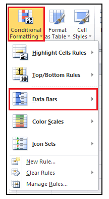
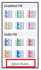
Data Bar Fill Type
As soon as you go to the Conditional Formatting Dara Bar section, Excel will option a secondary window displaying the two sets of Data Bar options, i.e., Gradient Fill and Solid Fill. Both have distinctive features and make your bars look more visually appealing.
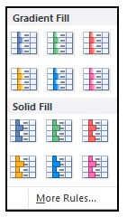
- Solid Fill: The users may opt for the Solid Fill data bars option if the numeric data values are hidden in the cells and only the bars are show
- Gradient Fill: The users shout opt for the Gradient Fill data bars option if the cells’ numeric data values are visible. The lighter colors at the end of the gradient, the more readable the numeric data values inside the cell are.
NOTE: IF you are inserting data bars along with the numeric data values, change the numbers to Bold font, so they are more readable.
If none of the above options fits your requirement, you can click on the ‘More Rules’ option and create some conditions to insert data bars. Using ‘More Rules’, you can also create your own customized bar charts with 2-colored bar or 3-colored bar, add borders to it, and perform other different styling options as well.
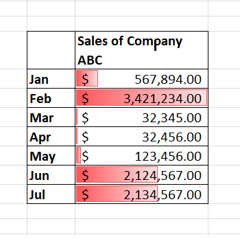
Example #1 – Implement Data Bars along with the Values in the below Monthly Sales table in your Excel worksheet
| Sales of Company ABC | |
|---|---|
| Jan | $ 567,894.00 |
| Feb | $ 3,421,234.00 |
| Mar | $ 32,345.00 |
| Apr | $ 32,456.00 |
| May | $ 123,456.00 |
| Jun | $ 2,124,567.00 |
| Jul | $ 2,134,567.00 |
Data bars in Excel helps a user to visualize the numbers and help them to save time. They are very easy to implement in Excel worksheet. We will cover the step by step procedure for adding data bars along with values:
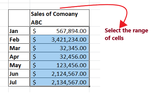
Step 1: Select the cells or range of cells
In your Excel worksheet, select the data range for which you want to add the data bars. Unlike, in our case we have selected the data cells D5 to D11.
Refer to the following image:
Step 2: Click on Conditional Formatting Highlight Cell Rules
- Go to the Home tab of the Excel ribbon. Click on the Conditional Formatting listed in the Excel ‘Styles’ group.
- It will open the following options window; click on the Data Bars option.

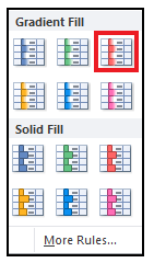
Step 3: Select the Data Bar Fill Type
- As soon as you click on the Data Bars, another secondary window appears, displaying the fill types.
- Since we want to go with Gradient color options, So we will choose the Gradient Fill type and will select a certain color option.
Refer to the below image.
NOTE: You can also click on more rules, to edit and format the existing data bars rules, bar appearance (color, size, format style, value) format the cell on the basis of their values, etc.
Step 4: Data Bars will be inserted in your worksheet
In the given Monthly Sales Report Excel table, all the cells will be inserted with data bar whose length depends on their values.
Look out in the below given image for the resulting output:
Wow!! The data cells look good and are visually more appealing. But wait, we have more impressive graphics which display the data bars inside the respective cell itself. In the following tutorial, we will cover more advanced examples.
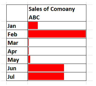
Example #2 – Implement Data Bars in your Excel Worksheet without the Values (Showing only bars, no numbers)
Here, we have twisted a question a bit. Now, we will insert data bars with the cells of your Monthly Sales Report table without their value. We will use the same Excel table (refer to the above monthly sales report Excel Table).
Showing data bars inside your cells is not the only part of the Data bar technique; it has many more interesting modules. In our case, since we do not want to see values but want to see only data bars in the table cells, we can select to show only bars instead of displaying both bars and numeric values.
To show only bars, you can follow the step-by-step procedure in your Excel worksheet:
Step 1: Select the cells or range of cells
In your Excel worksheet, select the data range for which you want to add the data bars. Unlike, in our case we have selected the data cells D5 to D11.
Refer to the following image:
Step 2: Click on Conditional Formatting Highlight Cell Rules
- Go to the Home tab of the Excel ribbon. Click on the Conditional Formatting listed in the Excel ‘Styles’ group.
- It will open the following options window; click on the Data Bars option.
Step 3: Select the Data Bar Fill Type
3. As soon as you click on the Data Bars, another secondary window appears, displaying the fill types.
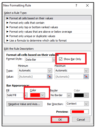
4. Since we have asked to insert bars without their values in the question. Since the direct option to show bar without value is not available, therefore we will click on the ‘More Rules’ option.
Refer to the below image.
Step 4: Select bar with no values option
1. As soon as you click on the ‘More Rules’, it will option the New Formatting Rule window box.
2. In the ‘Edit to Rule Description’ section, you will find the show bar only checkbox. Using your mouse cursor mark the tick on it.
3. Next, from the Bar appearance section, we will change the colors of the bars to red.
NOTE: You can customize the bars and make it visually more appealing, but adding borders, changing the colors, etc.,
4. Once done, click on OK.
Step 5: Excel will insert data bars without numeric values
In the given Monthly Sales Report Excel table, the data bars will be implemented with solid red color in the cells without their numeric values.
Look out in the below given image for the resulting output:
Example #3 – Using the Conditional Formatting data bars represent the various Negative Numbers in your data worksheet.
Excel Data bars can show only the negative numbers as well in your Excel worksheet. In the below-given table, we have the exam scores for seven different students because competitive exams have negative markings as well, so few of the students have scored negative marks as well.
| Name of the student | Exam Scores |
|---|---|
| Rahul | 56.00 |
| Varun | -6.00 |
| Himanshu | 21.00 |
| Tina | 34.00 |
| Jackeline | 56.00 |
| Soheir | 21.00 |
| Mohammed | -8.00 |
By directly looking at the Excel data, no one can instantly tell which student scored negative marks in the competitive exams. For this, you have to focus on the sheet. We require highlighting the negative numbers to identify the scores in each exam quickly. The Data Bar technique in conditional formatting functions to fulfill the above requirement.
Step 1: Select the cells or range of cells
In your Excel worksheet, select the data range for which you want to add the data bars. Unlike, in our case we have selected the data cells D5 to D11.
Refer to the following image:

Step 2: Click on Conditional Formatting Highlight Cell Rules
- Go to the Home tab of the Excel ribbon. Click on the Conditional Formatting listed in the Excel ‘Styles’ group.
- It will open the following options window; click on the Data Bars option.
Step 3: Select the Data Bar Fill Type
- As soon as you click on the Data Bars, another secondary window appears, displaying the fill types.
- Since we want to go with Gradient color options, So we will choose the Gradient Fill type and will select a certain color option.
Refer to the below image.
NOTE: You can also click on more rules, to edit and format the existing data bars rules, bar appearance (color, size, format style, value) format the cell on the basis of their values, etc.
Step 4: Data Bars will be inserted in your worksheet
In the given Score chart, all the cells will be inserted with data bar whose length depends on their values. For negative values are chart will be drawn away from the axis.
Look out in the below given image for the resulting output:


