Dynamic Arrays
Formula Example | Dynamic Array Functions | Old Array Formulas
Dynamic array formulas, entered into a single cell, fill multiple cells. This behavior in Excel 365/2021 is called spilling.
Formula Example
Let’s start with an easy example.
1. Fix the reference to cell E2 by placing a $ symbol in front of the column letter and row number.
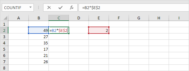
2. To quickly copy the formula in cell C2 to the other cells, select cell C2, click on the lower right corner of cell C2 and drag it down to cell C7.
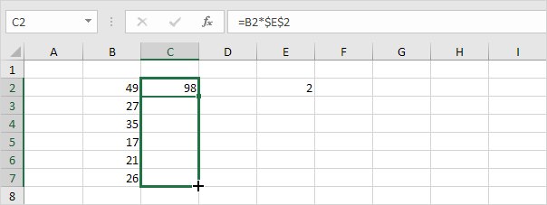
Check:
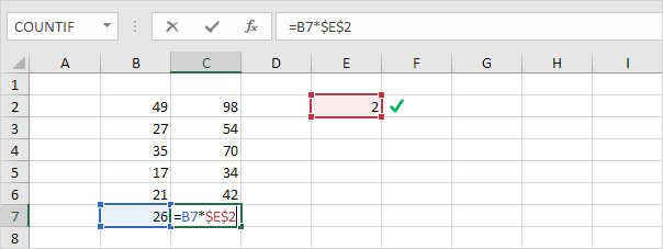
Explanation: the absolute reference ($E$2) stays the same, while the relative reference (B2) changes to B3, B4, B5, B6 and B7.
3. If you have Excel 365 or Excel 2021, simply enter the dynamic array formula shown below into cell C2.
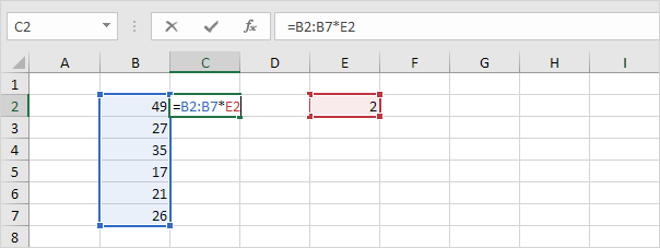
4. Press Enter.
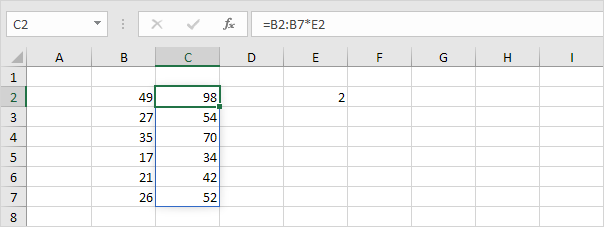
Explanation: this dynamic array (DA) formula, entered into cell C2, fills multiple cells. If you select a cell in the range C2:C7 a blue border appears.
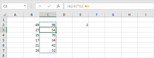
5. If you select a cell in the range C3:C7, the formula in the formula bar will be greyed out.
Dynamic Array Functions
Excel 365 and Excel 2021 offer many new dynamic array functions. Follow the links below to learn more about these functions.
1. The SORT function below sorts by the second column, in ascending order.
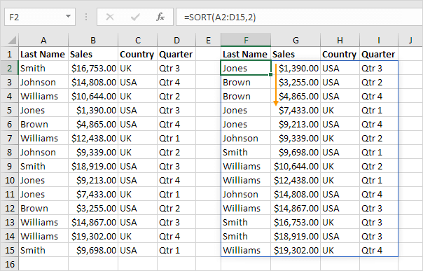
Note: this dynamic array function, entered into cell F2, fills multiple cells. Wow! This behavior in Excel 365/2021 is called spilling.
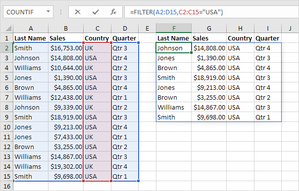
2. The FILTER function below extracts all USA records.
3. The RANDARRAY function below generates random decimal numbers between 0 and 1. The array below consists of 5 rows and 2 columns.

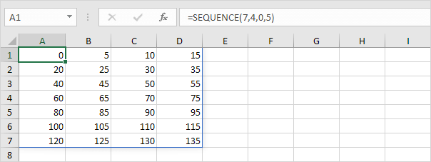
4. The SEQUENCE function below generates a two-dimensional array. Rows = 7, Columns = 4, Start = 0, Step = 5.
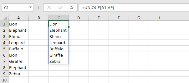
5. The UNIQUE function below (with no extra arguments) extracts unique values.
6. The XLOOKUP function below looks up the ID and returns the first name, last name and salary.
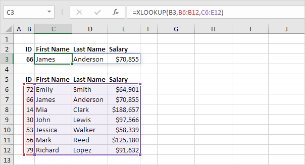
Note: if you have Excel 365 or Excel 2021, use XLOOKUP instead of VLOOKUP. The XLOOKUP function is easier to use and has some additional advantages.
Old Array Formulas
Old array formulas still work. The good news is, if you have Excel 365 or Excel 2021, you don’t have to press CTRL + SHIFT + ENTER anymore. Below you can find a few examples.
1. A traditional array formula finished by pressing CTRL + SHIFT + ENTER.
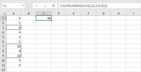
Explanation: this formula sums the 4 largest numbers.
2. The same formula in Excel 365/2021 finished by simply pressing Enter. Bye bye curly braces.
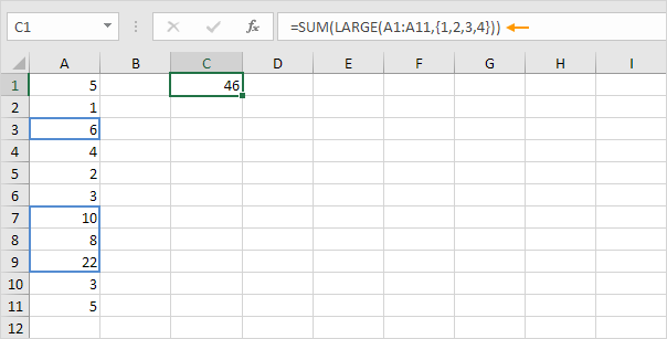
3. A traditional TRANSPOSE function entered by preselecting the range E2:E4 and finished by pressing CTRL + SHIFT + ENTER.

Explanation: the TRANSPOSE function converts a horizontal range to a vertical range, or vice versa.
4. The same function in Excel 365/2021, entered into a single cell, spills to neighboring cells.

Note: there’s much more to say about this topic so keep an eye on this page for more information.
Next Chapter: Sort


