

Excel Color Scales
Imagine how monotonous and tedious the job will be if you have to explore and analyze 500 items in your excel worksheet. Undoubtedly, it will be difficult to catch critical issues or locate the trends or patterns in the large chunks of data. But MS Excel conditional formatting tool acts as a savior for these cases. It helps the user highlight cells through different colors or emphasize unusual values and visualize the data using data bars, color scales, and icon sets, resulting in specific data variations.
Color scales represent all specialties such as temperatures, speed, ages, scores, etc. If you have large data in Excel that could benefit from this visual, it’s easier to execute than you might think.
Excel color scales allow the user to apply a gradient color scale in just minutes with conditional formatting. It presents two- and three-color scales with primary colors that the users can pick from and also the option to choose their customized colors.
What are Color Scales in Excel?
“The Color Scales in Excel are a part of conditional formatting used to highlight cells with different colors. The color scales option is applied to the respective cells according to the value in the cell specified. i.e., a dark color is applied if the cell value is higher, whereas a low light color is applied if the value in the cell is less.”
Color scales are very useful as it helps in proper data distribution and create variation in your Excel data, unlike different investment returns over time. The selected cells are colored with gradations of two color shades or three-color shades that fit minimum, midpoint, and maximum thresholds. These conditional formats color shades make it quicker to simultaneously compare the values of a range of cells.
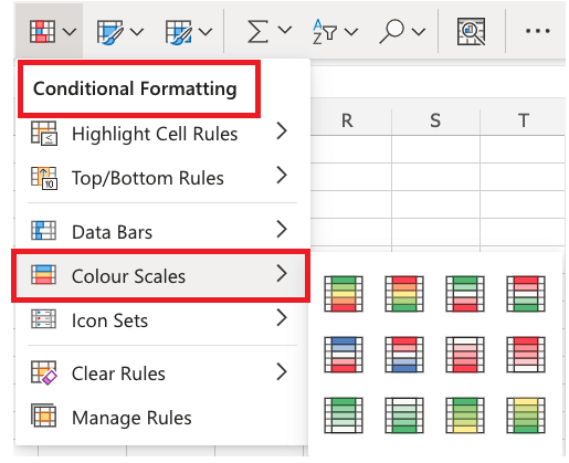
The Color Scales conditional formatting feature in Excel is found in the Conditional Formatting menu, typically listed in the ‘Styles’ group of the Home tab on the ribbon bar (refer to the below image).
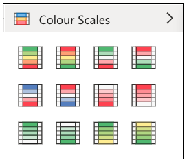
Microsoft Excel offers a few built color options with conditional formatting for color scales, so you can quickly apply the colors to your cells with a few clicks. It contains 6 two-color scales and 6 three-color scales options (refer to the below image). If you hover your mouse cursor over each color option, you will notice the arrangement of the colors in a screen tip. Excel will automatically highlight the selected cells with each color option. This is the quickest and most suitable method to select the color scale that best fits your Excel data.
Points to remember
- By default, Excel provides some inbuilt rules to apply the color shades within a few clicks quickly, but you can also create more customized rules.
- Conditional formatting color scales give you the result based on the specified conditions. If the conditions are matched, the color format will be applied to the selected cell; if the conditions are false, the selected cells are not formatted.
- If you hover your mouse cursor over each color scale option, you will notice the sequence of the colors in a screen tip. Excel will automatically highlight the selected cells with each color option.
- IF the selected range contains any blank cells or there are any other errors, Excel automatically skips to the next cell.
- The user can also delete or clear off the color scales for their worksheet.
- The Color Scale feature is not case sensitive.
Examples
Example 1: Excel Conditional Formatting Colour Scales Using default color options.
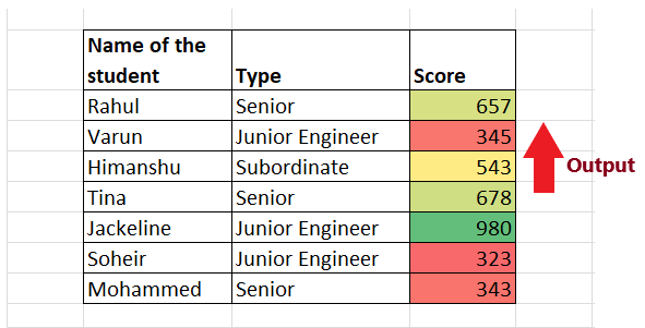
Below is the score table of various employees in a department examination test. Apply Excel Conditional Formatting color scales tool to highlight the cells with different colors based on their fetched scores.
| Name of the student | Type | Score |
|---|---|---|
| Rahul | Senior | 657 |
| Varun | Junior Engineer | 345 |
| Himanshu | Subordinate | 543 |
| Tina | Senior | 678 |
| Jackeline | Junior Engineer | 980 |
| Soheir | Junior Engineer | 323 |
| Mohammed | Senior | 343 |
Solution: Color scales allow users to apply a gradient color scale in just minutes with conditional formatting. Following are the steps using which you can implement different color shades in your select range of cells:
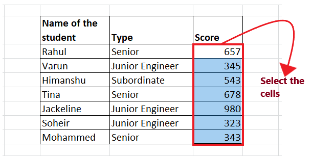
STEP-1 Select the cells
Select the entire cell or range of cells for which you wish to apply the color scales conditional formatting. In our case, we want to highlight all cells with the different gradients of colors based on their scores. So we have selected the cells ranging from E5 to E11.
Refer to the below image:
Step 2: Click on Conditional Formatting Color Scales
- Go to the Home tab of the Excel ribbon. Click on the Conditional Formatting
listed in the Excel style group. - It will open the following options window; click on the Color Scales option.


Step-3 Select any of the default formatting color
- As soon as you click on the ‘Colour Scales’ option Excel will open another window displaying the default color shades.
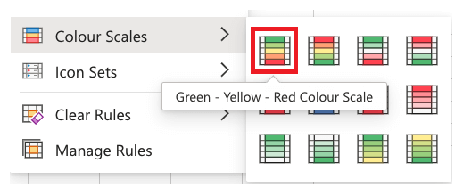
- It contains 6 two-color scales and 6 three-color scales options (refer to the below image). Select any of the colour option. In our case, we have selected the Gree-Yellow-Red Colour Scale.
NOTE: If you hover your mouse cursor over each color option, you will notice the arrangement of the colors in a screen tip. Excel will automatically highlight the selected cells with each color option.
Step-4 Excel will throw your result
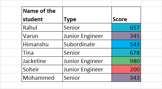
After completing the above steps, Excel will apply the three-color scales to the selected cells. The larger the cell values, the darker the color shade, whereas the lower the cell value, the lighter the color will be.
Refer to the below image for the resulting output:
The above output is fetched based on the default style. However, you can do the color formatting based on conditions as well. Let’s see in the next example how we can apply color scale formatting for a given condition.
Example 2 – Excel Conditional Formatting Colour Scales Using some conditions
Using the above score table (refer to the same table used in Example 1), format the cells of your score column if the cell value is greater than 600.
The conditional Formatting Color Scale option also allows you to format the cells based on some conditions. Following the steps to format the cells with different colours where the cell values are greater than 600:
STEP-1 Select the cells
Select the entire cell or range of cells for which you wish to apply the color scales conditional formatting. In our case, we want to highlight all cells with the different gradients of colors based on their scores. So we have selected the cells ranging from E5 to E11.
Refer to the below image:

Step 2: Click on Conditional Formatting Color Scales
- Go to the Home tab of the Excel ribbon. Click on the Conditional Formatting listed in the Excel style group.
- It will open the following options window; click on the Color Scales option.

Step 3: Select the ‘More Rules’ option
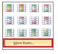
- As soon as you click on the Colour Scales, another secondary window appears, displaying the list of color options.
- Since in the questions, it’s mentioned to highlight cell value greater than 250. It means we have to specify a condition; therefore we will click on More Rules option.
Refer to the below image.
Step 4: Enter the Value for which you want to apply the condition
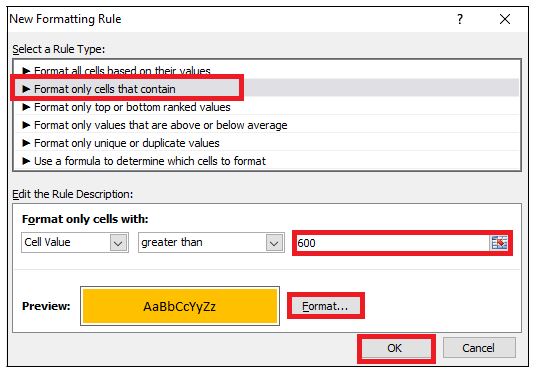
- The Conditional Formatting ‘New Formatting Rule’ dialog window will pop up.
- In the ‘Select a rule type’ option pane, select the text with ‘Format only cells that contain’
- As soon as you select this option, you will notice a change in the arrangement of ‘Edit the Rule Description’ window.
- In the first option select cell value
- In the second option, select greater than
- In the third option, specify 600 value in the textbox.
- Choose the required format for the Format option.
- Once done, click on OK.
Step 5: Excel will highlight the cells
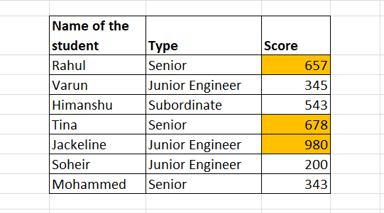
You will notice in the Score column, all the cells whose cell value is greater than 600 have been highlighted with the ‘Yellow’ color.
Refer to the below image for the resulting output:
Now since we have learnt how to apply colour formatting based on some conditions. Now, what if we want to edit the colour scale and want to insert our customized colours or, if necessary, how we can remove it.
How to Edit the Colour Scale in Excel
Although the color scale option is quite cool. But you can customize your table with new color options as well. All you need to do is to start with the first case, which is editing the colour scale.
Follow the below steps to quickly edit the colours for your table:
STEP-1 Select the cells
Select the entire cell or range of cells for which you wish to apply the color scales conditional formatting. In our case, we want to highlight all cells with the different gradients of colors based on their scores. So we have selected the cells ranging from E5 to E11.
Refer to the below image:

Step 2: Click on Conditional Formatting Color Scales
- Go to the Home tab of the Excel ribbon. Click on the Conditional Formatting listed in the Excel style group.
- It will open the following options window; click on the Color Scales option.

Step 3: Select the ‘More Rules’ option
- As soon as you click on the Colour Scales, another secondary window appears, displaying the list of color options.
- Since in the questions, it’s mentioned to highlight cell value greater than 600. It means we have to specify a condition; therefore we will click on More Rules option.
Refer to the below image.
Step 4: Select your own colour scales
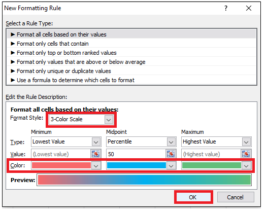
Scroll down to the ‘Edit the Rule Description’ window. In this section, can format all the cells based on their values:
- Format Style: You can choose whether you want it as a two-colour scale option or move with the three-colour scale.
- Next, you can pick specific 3 colours that suit you best. In our case, we’ll select this brilliant red for the minimum scale, intense blue for the midpoint scale, and medium green for the maximum scale of the range.
- Once done, click on OK.
Step 5: Color scale with customized color
As shown below, Excel will change the colours of the scales as per the specified 3-colour options.
How to Remove Color Scale in Excel
Sometimes you apply the color scales to highlight the cells and latter you need to remove the Color Scale from your Excel worksheet for sharing it across.
Follow the below steps to quickly remove the colors for your table:
- Select the entire cell or range of cells, for which you wish to apply the top/bottom rule conditional formatting.
- Go to the Home tab of the Excel ribbon. Click on the Conditional Formatting listed in the Excel style group. It will open the Conditional Formatting options window.
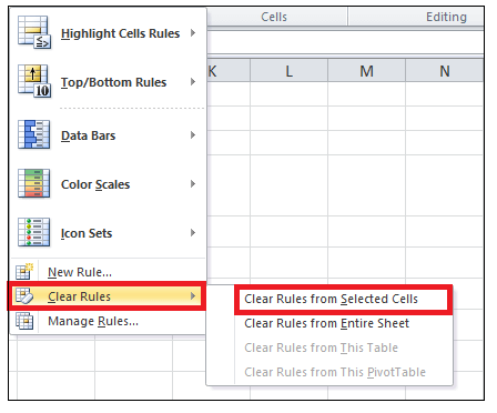
- Select ‘Clear Rules’ option from the ‘Conditional Formatting’ section.
- A dialog window will appear; click on ‘Clear Rules from Selected Cells’. You can choose another option (Clear Rules from the entire sheet) to remove formatting from the entire worksheet at once.
That’s it! The colour scale will be successfully removed from the selected cells of your Excel table.


