

Excel VLOOKUP Function
MS Excel, or Microsoft Excel, is powerful spreadsheet software with a distinctive range of built-in functions and formulas. Each function has a specific purpose and application. VLOOKUP is an extremely useful Excel function primarily used while working with advanced formulas within large data sets across sheets. Using the VLOOKUP function seems a little difficult for beginners and often leads to some unexpected errors in Excel. However, to become a master in Excel, we must learn the Excel VLOOKUP Function.

What is the VLOOKUP function in Excel?
In Excel, VLOOKUP stands for ‘Vertical Lookup‘, meaning the function only works vertically for the organized or structured table to be searched for the desired value. It is a built-in Excel function that searches for a specific value in the desired column to retrieve the respective value from a different column but on the same row. In simple words, the VLOOKUP function enables us to search for any specific piece of information within our worksheet while working with the large data sets.
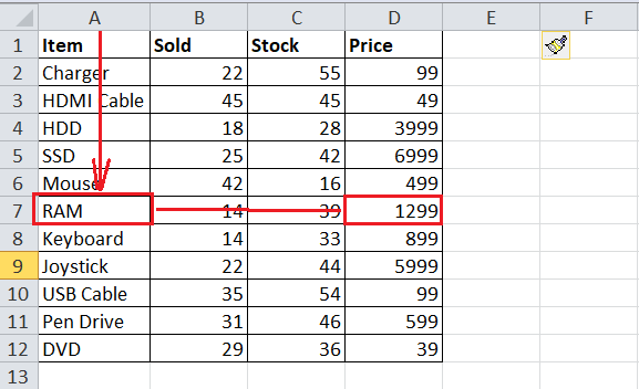
For example, the VLOOKUP function tells Excel to look for the desired piece of information (i.e., RAM) in the given data set or a range (i.e., table) and return some other respective information about that (i.e., the price of RAM).
The VLOOKUP function is available in Excel 2007, 2010, 2013, 2016, and other higher versions.
VLOOKUP Formula in Excel
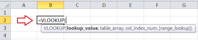
To enter a VLOOKUP formula in the desired cell (s), we need to type =VLOOKUP and select the function from the list by pressing the TAB key on the keyboard. After that, we can supply the respective arguments based on the syntax of the VLOOKUP.
Syntax of VLOOKUP
The syntax of the VLOOKUP function is defined as below:
Where, -lookup_value,” -table_array,” -col_index_num,” and -range_lookup” are the arguments of VLOOKUP function.
Arguments of VLOOKUP
The VLOOKUP function requires the following arguments in which the first three arguments are mandatory while the last argument (range_lookup) is optional:
Lookup_value
It is a required argument to specify the value we need to search for in the first column of the supplied table array or range. A lookup value can be in the form of any value like text, number, and date or the value obtained by any other function in the sheet. Unlike the numeric values or cell references, we must always enclose the text values within the straight double-quotes.
Table_array
It is another required argument used to specify the data array or a range of cells where the function will search for the lookup value. The function always looks up in the table array’s leftmost column (first column) and retrieves a corresponding match. The table array may contain multiple numeric values, text values, dates, and/ or logical values.
Col_index_num
Like the above two arguments, the col_index_num is also a required argument. It is specified as an integer to represent the number of a specific column from which we want to obtain the desired value. It must be selected from the supplied table array or a range only.
Range_lookup
It is an optional argument of the VLOOKUP function used to define what the function must return when it does not find an exact match to the lookup table. We can specify this argument as either TRUE or FALSE.
- TRUE: When the argument is set as TRUE, the function tries to find the approximate match in the event if no exact match is found. The function then finds the closest match below the lookup_table. We can also use ‘1’ to specify the argument as TRUE.
- FALSE: The function only tries to find the exact match when the argument is set as FALSE. The function returns an error if no exact match is found below the lookup_table. We can also use ‘0’ to specify the argument as FALSE.
How to use the VLOOKUP function in Excel?
After understanding the basics of the VLOOKUP function, using it in an Excel sheet becomes a little easier. The functionality of VLOOKUP is the same in all versions of Excel and even in other spreadsheet programs. To use the VLOOKUP function in our sheet, we need to perform the following steps:
Step 1: Organize the Worksheet Data and Type Formula Name.
We must organize or structure our sheet data properly. Since VLOOKUP only works in a left to right order, we must ensure that the value we want to look up is present in the left side column of the data we want to obtain.
Once the data is properly structured, we must select the resultant cell to record the retrieved value, type “=VLOOKUP(” without quotes, and follow the next step. It is recommended to select the VLOOKUP function from the function list to avoid misspelling the function name.
Step 2: Tell the Function What to lookup or search for.
After entering the function name and starting parenthesis, we need to select a cell or type the respective cell reference where the information we want to look up is recorded.
Step 3: Tell the Function where to look.
In the next step, we need to supply or enter the range or table where our effective data or value is present. By entering the table, we tell Excel to search in the leftmost column of this given data and find the information we want to look up.
Step 4: Tell Excel which column should be used to get the result.
After supplying the effective data range or table, we must specify the column number to tell Excel to extract the data we want as an output via VLOOKUP. The column number is written or specified in a general numeric form. For example, if our output data is present in the 2nd column of the supplied table/range, we must specify the column number like 2 in the formula.
Step 5: Tell Excel whether to find an Exact or Approximate Match.
Lastly, we must tell Excel whether we want to lookup for the exact match or approximate match. We must enter TRUE (or 1) for an approximate match and FALSE (or 0) for the exact match. For example, when we want to lookup for any ID or word, it is better to use an exact match. In contrast, the approximate match is useful when looking for an exact figure that may not typically be present in the table.
Let us understand the working of the VLOOKUP function better with the help of examples:
Examples
Let us discuss examples to look for values in exact and approximate matches using VLOOKUP:
Example 1: Exact Match in VLOOKUP
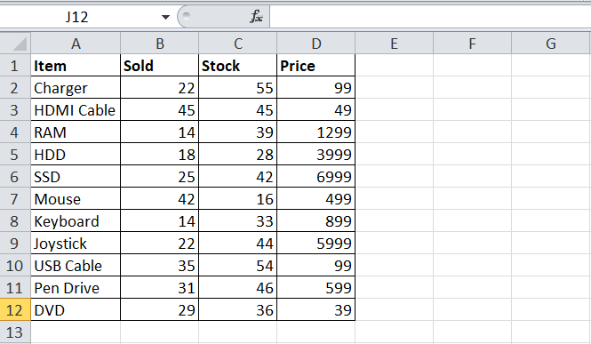
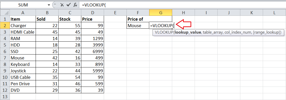
Consider the following excel sheet as an example where we have data containing a list of some items with their prices. We need to use VLOOKUP to find the price of any specific item (i.e., ‘Mouse’) from the table.
We must perform the following steps to find the price of Mouse from our data table:
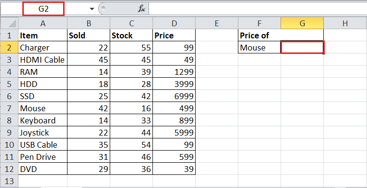
- First, we need to select a cell to record the price of the Mouse. In our example sheet, we select cell G2.

- After selecting a resultant cell, we start typing the VLOOKUP function starting with an equal sign and select from the function list by pressing the TAB key on the keyboard.
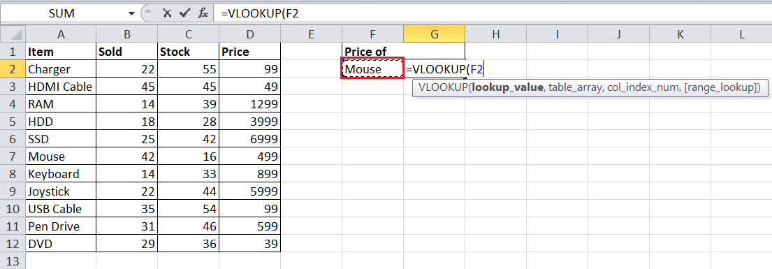
- Next, we select the cell with a value that we want to look up. We select or type the cell F2 in the VLOOKUP function as the first argument in our example.
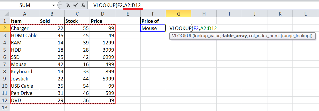
- After supplying the first argument, we type Comma (,) and select the range (or table array) in which we want to search for the lookup value and obtain the desired output. In our case, we select the range (A2:D12) without brackets.
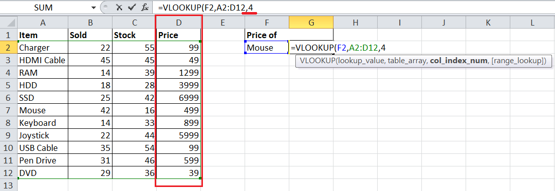
- After entering the range, we again type Comma (,) to separate arguments. After that, we need to type the column number within the supplied range in which we want to look up the output value. In our case, it is the price column, so we select type 4.
- Lastly, we enter the last argument as FALSE or 0 to find an exact match for the lookup value ‘Mouse’. After that, we type the ending parentheses and press the Enter key to obtain results.
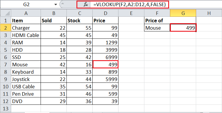
In our example sheet, we can change the item name in cell F2 and get the corresponding price for that item in real-time.
Example 2: Approximate Match in VLOOKUP
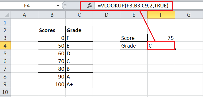
Consider the following excel sheet as an example where we have recorded data containing a list of scores with their respective grades. We need to use VLOOKUP to look up the value 75 and find the corresponding grade from the table.
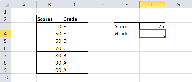
Since our table does not contain the value 75 in the leftmost column, we use VLOOKUP to return an approximate match. We must perform the following steps to find the nearest match (grade) for our lookup value (75) from our data table:
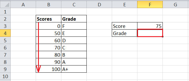
- First, we must sort the leftmost column of our data range in ascending order. It is essential when using the VLOOKUP function in an approximate match mode. After that, we need to select a cell to record a grade. In our example sheet, we select a cell F4.
- In the next step, we enter the VLOOKUP formula similar to the previous example. We first type “=VLOOKUP(” without quotes, select the cell with a lookup value (F3, in our case), select the data table (B2:C9, in our case), and type the column number (2, in our case) from which we want to retrieve the output.
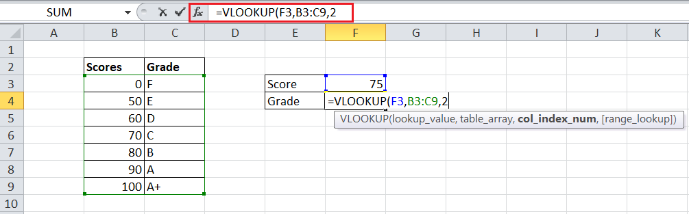
- Unlike the previous example, we now enter TRUE as a fourth argument. It tells the VLOOKUP function to return an approximate match when no exact match is found. In our case, the function does not find the lookup value 75 in the first column of the supplied range, so it returns the largest value smaller than 75. In our example sheet, the approximate match value is 70. Therefore, after pressing the Enter key on the keyboard, the VLOOKUP function returns the output grade C, which is the grade for score 70.
We can type other random scores (or numbers) to get their respective grades. If an exact match is found, the function will return its respective grade accordingly.
Limitations of VLOOKUP
Although VLOOKUP is a powerful function, it has certain limitations, i.e.:
VLOOKUP always looks right
One of the major limitations of the VLOOKUP function is that it cannot return the value or output from any of the left side columns of the lookup value. The function always works by looking up the value in the leftmost column of the selected table while returning the respective value from the desired column to its right.
For instance, consider the following sheet as an example data set where we have some employees’ names with their salaries.
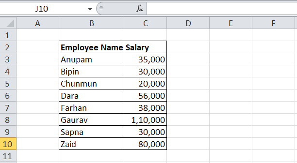
We can use the VLOOKUP function to find the salary of any desired employee in the following way:
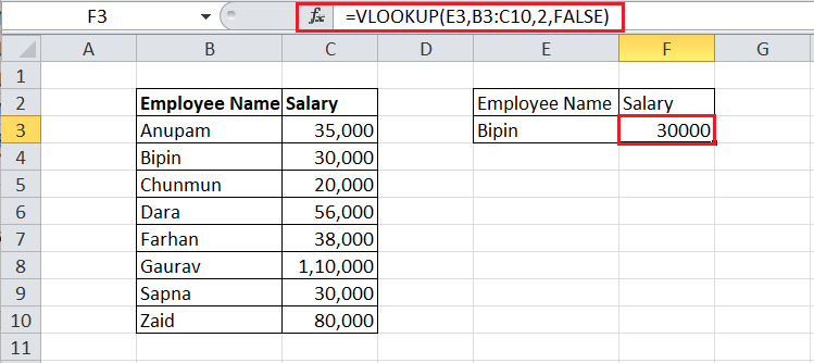
However, we cannot find the employee’s name based on his salary. The VLOOKUP function cannot use the salary as a lookup value while returning the value from its left side column. Instead, it will return an error.
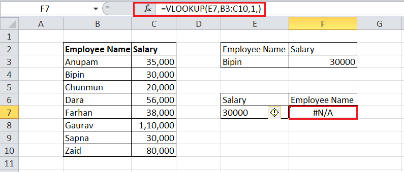
To use Left Lookup, we can use the combination of INDEX and MATCH functions in Excel.
VLOOKUP is Case-insensitive
The VLOOKUP function in Excel works in a case-insensitive way. This means the function treats uppercase and lowercase values equally when looking through the table. For instance, we will still get the results if we try to lookup an employee name in the UPPERCASE (i.e., BIPIN).
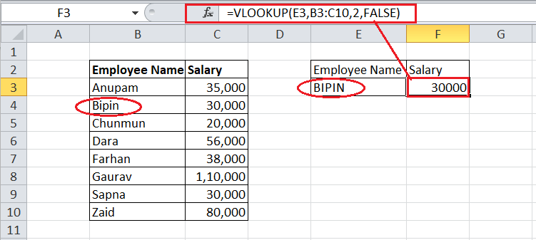
Since VLOOKUP is case-sensitive, it will work the same for lookup values BIPIN, Bipin, bipin, bipiN, etc.
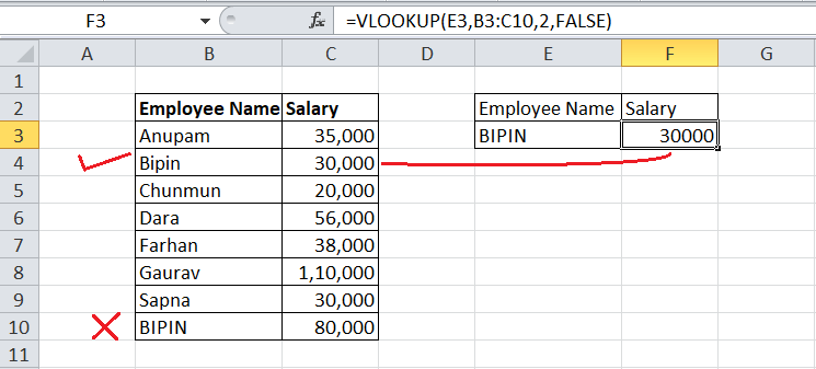
VLOOKUP always finds the first match
The VLOOKUP function always produces a result for the first lookup value it finds vertically in a table column. If there are duplicates in the column, all such values will be ignored. For example, the VLOOKUP function returns the salary for the employee name ‘Bipin’ from cell B4, not from B10. It is because the function always matches the first instance and is case-insensitive.
Excel VLOOKUP Errors
When using VLOOKUP in Excel, we often encounter unexpected errors instead of the desired results. Some such errors include the #N/A, #NAME?, #REF!, and #VALUE!.
- VLOOKUP #N/A Error: It primarily occurs when the lookup value is misspelled or not present in the selected table, the lookup column is not the leftmost column, hidden spaces in lookup values, and/ or numerical values are formatted as texts.
- VLOOKUP #NAME? Error: It occurs when the function name is misspelled or wrong.
- VLOOKUP #REF! Error: It occurs when the column number (col_index_num) is higher than the range selected.
- VLOOKUP #VALUE! Error: It mainly occurs when the lookup value contains more than 255 characters, missing parameters/ arguments, and/ or column number (col_index_num) is below 1.
Important Points to Remember
- If we do not specify range-lookup in VLOOKUP, the function returns an exact match if it exists; otherwise, non-exact (approximate) match.
- If the sheet already has the VLOOKUP formula, it is recommended not to insert a new column or delete an existing column in the table range. When we insert/delete a column in the table, the column index number does not change accordingly, resulting in incorrect results or an error.
- VLOOKUP can lookup values with signs or symbols. For example, an asterisk (*), question mark (?), etc.


