Excel XIRR Function
Calculating cash flows at intervals is a routinely task followed in every industry, business or services. Similarly, estimating the internal rate of interval is essential to maintain the cash flow. To make your task easier, Excel has introduced an inbuilt function known as XIRR function.
In this tutorial, you will learn what is XIRR function, its syntax, parameter, points to remember, how this formula works and various examples by using the XIRR function to calculate the internal rate of return for a series of cash flow.
What is XIRR function?
“The Excel XIRR function in an inbuilt function used to calculate the internal rate of return for a series of cash flows that happen at irregular intermissions. In this function, the payments are viewed as negative figures and income as positive figures. If the initial value is a cost or payment, it must be a negative value. Subsequent payments are discounted based on a 365-day year.“
XIRR is works in the similar method of inbuilt XNPV function. The Excel XIRR function returns the interest rate when XNPV = 0. This function uses iteration to reach at a conclusion. Though, initially it starting with guess (which defaults to 0.1 or 10% if the armament is omitted) XIRR iterates through a calculation until the output attain an accuracy level of 0.000001 percent. If it didn’t find any output even after 100 tries, this function returns the #NUM! error. If you want to calculate the internal rate of return for a sequence of regular, periodic cash flows, using the inbuilt IRR function is suggested.
The function takes three parameters i.e., values, dates, and guess. The argument Values represent a series of cash flows. The first number value represents to a cost at the start of any investment. If the first payment is a cost, it must be supplied as a negative number. Values must contain at least one negative and one positive number, else the XIRR will return a #NUM! error. If mistakenly the values parameter includes any non-numeric data, XIRR returns a #VALUE! error. Sometimes the XIRR function returns #NUM!, even when you have used at least one positive and one negative value in the values parameter. For such cases, try different ratios to guess between 0 and 1.
The dates parameter signifies the corresponding dates in a proper format that can later be converted to values. However, the supplied date values must be valid Excel dates. You need not supply the dates in chronological order. Typically, dates are entered as a range. If the supplied date values are recognized as a date by Excel, the XIRR function returns a #VALUE! error.
Syntax
=XIRR (values, dates, [guess])
Parameter
Values (required) – This parameter represents the array or reference to cells that contain cash flows.
Dates (required) – This argument represents the dates that match to cash flows, in any order. Dates do not need to be entered in chronological order. Typically, dates is supplied as a range. If any date is not recognized as a date, XIRR returns a #VALUE! error.
Guess [optional] – This argument represents an estimate value for expected XIRR. If this parameter is omitted, by default this function takes 0.1 (10%).
Return Value
The XIRR function in Excel returns the calculated internal rate of return.
XIRR – Things to Remember
Before working on Microsoft Excel XIRR Function, make sure to go through with the below facts:
- All the entered values array must contain at least one positive value and one negative value.
- The specified dates must be valid Excel dates that can be converted to values
- The provided dates do not need to be in chronological order.
- The XIRR function is related to the Excel XNPV function.
- The XIRR function also throws the #NUM! error if either of the situation occurs:
- If the specified values and dates arrays are of diverse lengths;
- If the specified array values do not contain at least one positive and one negative value;
- If any of the specified dates precede the first date (the value of after date values are smaller than the first one);
- If the calculation fails to converge after 100 iterations.
- The XIRR function throws the #VALUE! error in Excel when either of the specified dates cannot be recognized by Microsoft as valid dates.
Examples:
#XIRR Example1: Calculate the investment using the XIRR function for the given project.
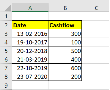
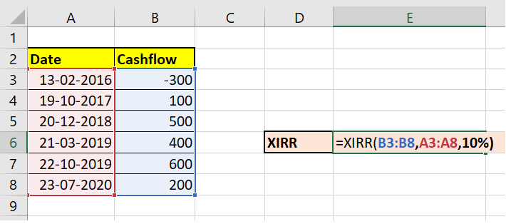
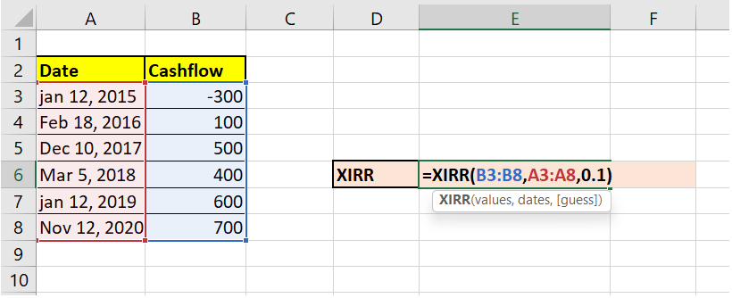
The below sheet shows that a company started a project on Feb 13, 2016. The project gives us cash flows the following year; again, it received a cash flow towards the end of 2018, after 3 months, then at the end of 2019, and annually after that. The data given is shown below:
Follow the below-given steps to calculate internal rate of return for irregular cash flows using the Excel XIRR () function:
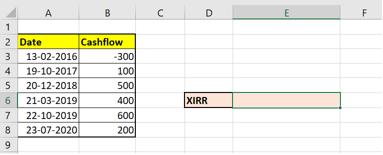
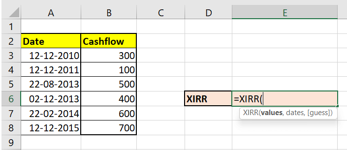
Step 1: Select a cell to calculate XIRR
Place your mouse cursor to a cell from where you want to have the result of XIRR() fun. In our case, we have selected cell E6 of our Excel worksheet.
Refer to the given below image:
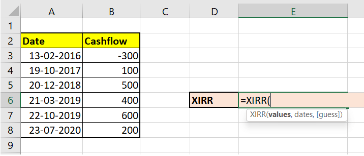
STEP 2: Type the XIRR function
In E6, we will start typing the function with the equal to (=) sign followed by the XIRR function. Therefore, our function will become: = XIRR(
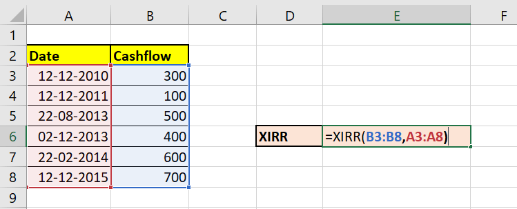
STEP 3: Insert all the parameters
- At first, this function will ask you to specify the values parameter. Here, we will specify the cash flow values. Make sure the array must contain at least one positive value and one negative value. The formula will be = XIRR(B3:B8,
- The next argument is Dates. This parameter should contain all the dates in an chronological order. The formula will be = = XIRR(B3:B8, A3:A8,
- The next argument we will specify an estimate value for expected XIRR. So here we will give a value of 10%. The formula will be = XIRR(B3:B8, A3:A8,10%)
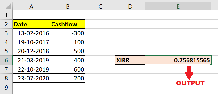
Step 4: The XIRR function will return the output
As a result, the XIRR function will return the value of the given investment for the above project that does not have regular periodic cash flows.
#XIRR Example2: Example to demonstrate XIRR not working.
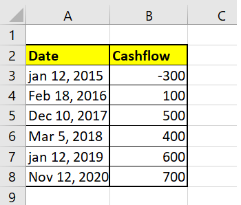
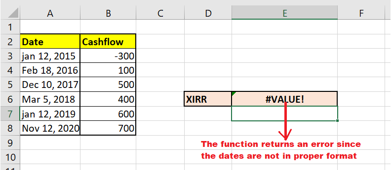
In the below datasheet, you will notice the dates are not in proper order. They are manually typed, though the meaning is correct, and the user can properly understand them. Microsoft Excel won’t recognize this date order since they are not in its valid format. The data is shown below:
Follow the below-given steps to calculate internal rate of return for irregular cash flows using the Excel XIRR () function:
Step 1: Select a cell to calculate XIRR
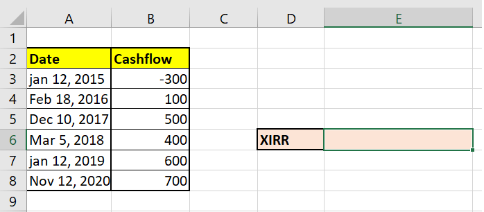
Place your mouse cursor to a cell from where you want to have the result of XIRR() fun. In our case, we have selected cell E6 of our Excel worksheet.
Refer to the given below image:
STEP 2: Type the XIRR function
In E6, we will start typing the function with the equal to (=) sign followed by the XIRR function. Therefore, our function will become: = XIRR(
STEP 3: Insert all the parameters
- At first, this function will ask you to specify the values parameter. Here, we will specify the cash flow values. Make sure the array must contain at least one positive value and one negative value. The formula will be = XIRR(B3:B8,
- The next argument is Dates. This parameter should contain all the dates in an chronological order. The formula will be = = XIRR(B3:B8, A3:A8,
- The next argument we will specify an estimate value for expected XIRR. So here we will give a value of 10%. The formula will be = XIRR(B3:B8, A3:A8,10%)
Step 4: The XIRR function will return the output
As a result, the XIRR function will return the #value error because Microsoft cannot recognise the specified date format.
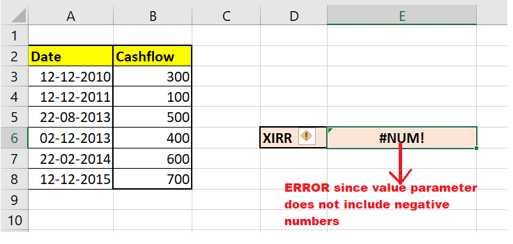
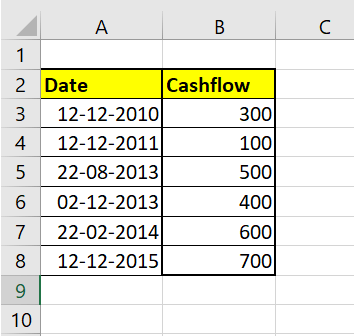
#XIRR Example3: Example to demonstrate if the value array don’t contain a positive or negative value.
Follow the below-given steps to calculate internal rate of return for irregular cash flows using the Excel XIRR () function:
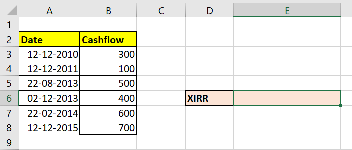
Step 1: Select a cell to calculate XIRR
Place your mouse cursor to a cell from where you want to have the result.
STEP 2: Type the XIRR function
In E6, we will start typing the function with the equal to (=) sign followed by the XIRR function. Therefore, our function will become: = XIRR(
STEP 3: Insert all the parameters
- At first, this function will ask you to specify the values parameter. Here, we will specify the cash flow values. The formula will be = XIRR(B3:B8,
- The next argument is Dates. The formula will be = = XIRR(B3:B8,A3:A8,
Step 4: The XIRR function will return error as an output
As a result, the XIRR function will return the #num error because the value argument must contain atleast one positive and one negative number. Sometimes the XIRR function returns #NUM!, even when you have used at least one positive and one negative value in the values parameter. For such cases, try different ratios to guess between 0 and 1.