Format Cells in Excel

MS Excel, short for Microsoft Excel, refers to a powerful spreadsheet software developed by Microsoft to help users record data within the cells across multiple worksheets. By default, the structure and appearance of the worksheet are basic, and each cell follows the same settings. However, Excel offers various options to format cells as per our choice. Although it is an optional step in most cases, it can help us make our worksheet effective and productive in distinct ways.

This article discusses the brief introduction of the Format Cells in Excel and how we can take advantage of it in our Excel worksheet. Each cell can be formatted or modified with an entirely different appearance as desired by the user.

What is Format Cells in Excel?

The Excel’s Format Cells feature allows users to adjust or modify the formatting of one or more cells and/or their values’ appearance in the sheet, but without changing the number themselves. The Format Cells provide various control options that enable users to change the view of the displayed data within the cells.

We can use the Format Cells to change the date style time style, add/ remove colors in fonts or background, insert the border of a specific style, protect the cells, and many more. Using Excel formatting, we usually add finishing or final touches to prepare and present the data accurately.

For example, suppose we have a worksheet with extremely large data, including some dates and prices. We can add currency signs (e.g., $) to cells containing prices and configure dates format to represent standard dates (xx/xx/xxxx). In this way, cells’ formatting helps us draw attention to certain data and highlight essential content. However, there are various formats under the Format Cells window.

Accessing the Format Cells

There are several options for accessing or opening the Format Cells dialogue box in Excel. Such options include the ribbon, contextual menu (right-click menu), and keyboard shortcuts.

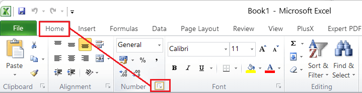
• Using the Ribbon: The ribbon is the centralized area located on the top of the Excel window. It consists of most Excel tools and features. When opening the Format Cells dialogue box, we need to go to the Home tab and click the More icon from the bottom-right corner of the Number formatting group.
  
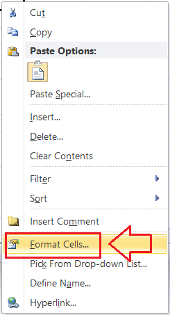
• Using the contextual Menu: The contextual menu refers to the right-click menu. We can press the right-click on the desired Excel cell(s) using the mouse and choose the Format Cells option to launch the Format Cells dialogue box.
  
• Using the keyboard shortcut: The keyboard shortcut is the fastest way of accessing the Format Cells dialogue box in Excel. We can use the shortcut ‘Ctrl + 1‘ inside the Excel window to open the Format Cells dialogue box. However, we must press the key ‘1’ from the numeric row in the keyboard area and not from the number pad.
  

What are the elements of the Format Cells window?

Elements of the Format Cells window refer to the tabs in its dialogue box. Typically, the Format Cells window or Format Cells dialogue box has six tabs which are discussed below:

Number Tab

The Number tab provides various formats to change the appearance or formatting of numeric values within cells. This usually changes the way numbers are displayed in cells without changing the exact values.

The following are the available or existing number formats in Excel:

General

In Excel, the General is the default format style. Whenever we create a new Excel sheet, each worksheet cell follows the General format. According to this Format, Excel automatically identifies the values entered in corresponding cells and displays them by guessing the best suitable format.

For instance, suppose we have an Excel cell with the ‘General’ formatting. If we enter any number like 2-3 in the cell, Excel reads the value as a date and converts it to a short date format like 02-Mar. If we select the particular cell and check the formula bar, Excel displays the complete date in the 02-03-current year (i.e., 2022) format.

If we do not want Excel to convert the entered value to date, we must specify the other format required to display the value.

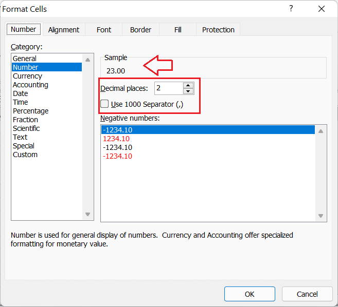
Number

As the name suggests, the ‘Number‘ format displays the entered values in the form of numerical values. It also adds the decimals with given values, even if we don’t manually type them.

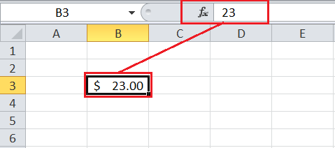
For instance, suppose we set an Excel cell with the ‘Number’ formatting. If we enter any number like 23 in the cell, Excel reads the value as a numeric value and changes its view by adding the decimals like 23.00. In particular, the ‘Number’ format sets the cell(s) to display numbers in a general form.

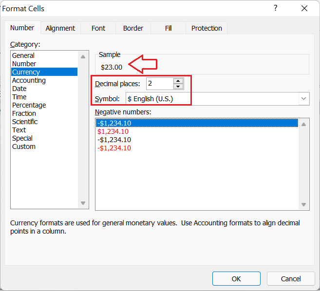
Currency

The Currency format is a specific Excel format used especially for currency values like prices in cells. The Currency format adds a currency sign (such as $, €, ?, etc.) before the values that are entered in the corresponding cells. By default, Excel adds the currency sign according to the selected geographic region; however, it can be changed accordingly.

For instance, suppose we set an Excel cell with the ‘Currency’ formatting. If we enter any number like 23 in the cell, Excel reads the value as a currency and changes its view by adding the currency sign like $23.00. The Currency format is most commonly used to represent general monetary values within the Excel cells.

Accounting

Excel’s Accounting format is the same as the Currency Format. This particular format is also used to display entered values in the form of monetary values. But, it is slightly different from the Currency format in a way that it aligns or lines up the currency sign and decimals in corresponding columns. Using the Accounting format, we can make it easier for viewers to read or understand a huge list of currency values.

In the above image, the currency symbol is aligned to the left because of the Accounting format, while the Currency format appends it before the corresponding value without any alignment.

Date

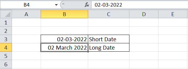
The Date format is used to represent given or entered numbers in the form of dates. Typically, we use the short date and long date formats in Excel. The short date format represents the given numbers as DD-MM-YYYY, whereas the long date format represents the same as DD MONTH YYYY. In Excel, we can select between various date formats from the Format Cells dialogue box. We only change the view using different date formats, but not the dates.

Time

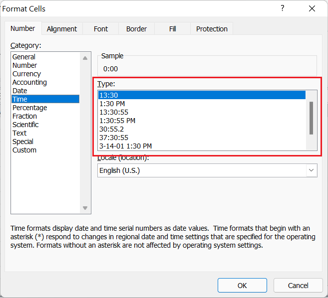
The Time format is used to represent the entered values or numbers in the form of time. It usually displays numbers in the form of HH/MM/SS, where HH means hours, MM means minutes, and SS means seconds. Also, the time format can add AM (Ante Meridiem) or PM (Post Meridiem) depending on the selected date format, such as 12 hours format or 24 hours format. We can select between various time formats from the Format Cells dialogue box. For example, 1.30 PM, 13.30, etc.

Percentage

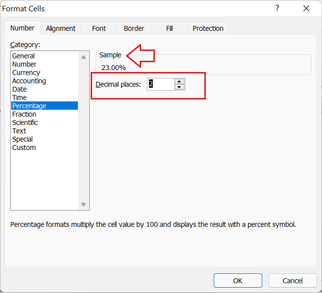
The Percentage format helps us display entered numbers as percentages with decimal places. This particular format adds the percentage sign (%) at the end of a given value within the cell. Also, the decimal places are automatically added with values. By default, the decimals are added up to two digits. However, we can change it accordingly.

For instance, suppose we set an Excel cell with the ‘Percentage’ formatting. If we enter any number like 0.23 in the cell, Excel reads the value as a percentage and changes its view by adding the percentage sign and decimals like 23.00%.

Fraction

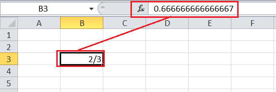
When a user enters any fraction in an Excel cell, the value automatically changes to dates or decimals. Excel auto-adjust the entered value by guessing the best suitable cell format. Using the fraction format can prevent Excel from automatically changing the fraction in the desired cells. The fraction format uses a forward slash while displaying the numbers within the cells.

For instance, when we enter any fraction like 2/3 in an Excel cell, it changes to 02-Mar. But, if we set that particular cell as a fraction, the number entered will not be changed and will appear as supplied, i.e., 2/3.

Scientific

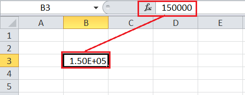
The Scientific format allows users to set the desired Excel cell(s) as a reference to scientific notation, which means an exponential form. When a user enters a too large number, the Excel automatically converts the corresponding number or a cell in scientific notation.

For instance, suppose we set an Excel cell with the ‘Scientific’ formatting. If we enter any number like 1,50,000 in the cell, Excel reads the value as a large integer and changes its view by converting it to a scientific notation like 1.50E+05.

To restrict Excel from automatically changing large integers into the scientific format, we can set the cell as ‘Number’ or other desired format.

Text

The Text format helps users set the desired cell (s) as text only. It keeps the entered values formatted as normal text. No matter what we enter into cells, it will display the same values as they were supplied. Excel uses the Text format automatically when a user enters both text and number s within the Excel cell. Text format does not participate in calculations when using formulas or functions for corresponding cells.

For example, suppose we set two Excel cells (B3, B4) as ‘Text’ format. We enter the numbers in both cells. When we try to add the numbers of both the cells in another cell (B5), it does not provide the expected result. This is because numbers are displayed as numeric values, but they are text values because the corresponding cells are formatted as text.

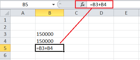
The sum is not visible in the above image because the text values cannot be added together.

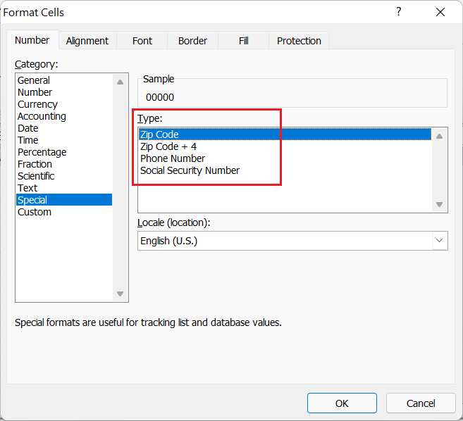
Special

The Special Format represents the entered values or numbers with special formatting. This number format is mainly used for ZIP codes, additional four-digit ZIP codes, telephone numbers, and Social Security numbers. The Special format helps to tracklists and database values easily.

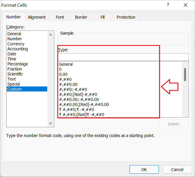
Custom

Although Excel has many predefined number formats, there may be chances when we might need to use a specific format that is not present in Excel. We can take advantage of the Custom Number Format of Excel in such a case. Using the Custom format, we can create any desired number format for selected cells. To create a custom format, we must specify the format code using the appropriate structure. Excel also displays existing format codes to be used as a starting point for a custom number format.

Alignment Tab

The Alignment tab provides various formatting options to align the cell values in the worksheet. This usually changes the way the values are aligned in cells without changing the exact values. Using this tab, we can typically choose between horizontal or vertical alignments, text direction, orientation, and some text controls.

The following are the available or existing options/settings along with their details that we can access from the Format Cells window in Excel:

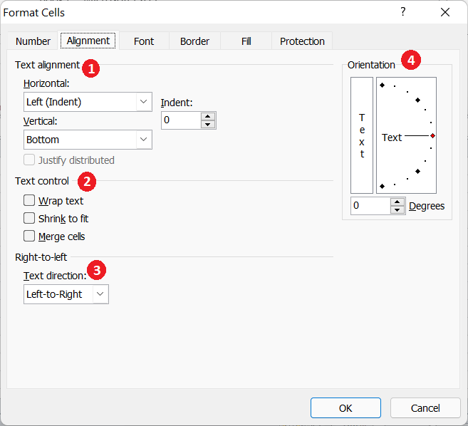
1. Text Alignment: Using the text alignment section, we can choose to align the cell’s contents in a horizontal axis and/or vertical axis. The horizontal alignment drop-down gives access to alignments like left, right, center, fill, justify, etc. Besides, the vertical alignment drop-down gives access to alignments like top, center, bottom, justify, etc. Moreover, we can use the Indent box to increase/decrease the margin between the text and the cell border.
2. Text Control: Using the text control section, we can choose options like wrap text, shrink to fit, and merge cells. The ‘wrap text’ option helps make the cell content visible by displaying it on multiple lines. The ‘merge cells’ option helps to join multiple cells into one larger cell. The ‘shrink text’ option helps make the cell content visible by changing its size within the cell.
3. Text direction: Using the text direction section, we can choose a text direction between the context, left-to-right, and right-to-left.
4. Orientation: Using the orientation section, we can choose to rotate the cell content at any desired angle. We can define or enter the desired rotation angle in the box before Degrees.

Font tab

The Font tab provides various formatting options that help adjust fonts for cell values in the worksheet. This usually changes the way the fonts are displayed in cells without changing the exact values. Using this tab, we can typically modify appearance like the font style, size, color, etc.

Following are the available or existing options/settings to modify fonts, which we can access from the Format Cells window in Excel:

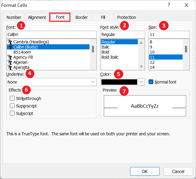
1. Font: Using the Fonts section, we can choose between different designs of installed fonts to be applied to the selected Excel cells.
2. Font style: Using the Font style section, we can choose a different style like bold, italic, etc.
3. Size: Using the Size section, we can choose the font size to be displayed within the selected Excel cells. If we don’t find a suitable font size (i.e., 13) in the list, we can type the desired size in the box and press the Enter key.
4. Underline: Using the Underline section, we can choose to add an underline below the fonts or texts within the cells. The drop-down lists additional underline preferences like a single line, double-line, etc.
5. Color: Using the Color section, we can choose to apply colors on fonts within the selected cells. We can select existing colors or choose our custom desired color.
6. Effects: Using the Effects section, we can choose font effects between Strikethrough, Superscript, and Subscript.
7. Preview: The preview section displays the changes selected for the fonts.

Border tab

The Border tab provides various formatting options that help add/remove the border in one or more sides of the cell in the worksheet. The section also allows us to choose the border line style and color.

Following are the available or existing options/settings to adjust borders, which we can access from the Format Cells window in Excel:

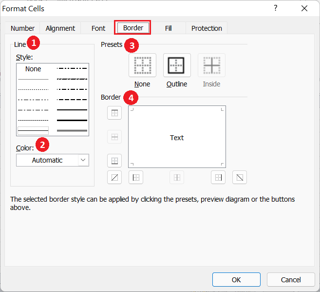
1. Style: Using the Style section, we can choose between various styles of lines to use as borders on the desired cells. It displays many border styles like dashed, dotted, bold, etc.
2. Color: Using the Colors section, we can choose between the various existing colors used for the borders.
3. Presets: Using the Presets section, we can choose between three predefined border combinations, such as None (no borders), Outline (all sides borders), and Inside (borders in connecting grid lines of multiple cells).
4. Border: Using the Border section, we can choose to add a border in any particular side like the top, bottom, left, right, diagonal, etc.

Fill tab

The Fill tab provides various formatting options for filling colors in the background area of cells in the worksheet. The section provides existing colors that we can choose from. In addition, we can choose to make custom colors. Excel also has some preferences for adding patterns and effects to the background of cells.

Following are the available or existing options/settings to adjust colors, which we can access from the Format Cells window in Excel:

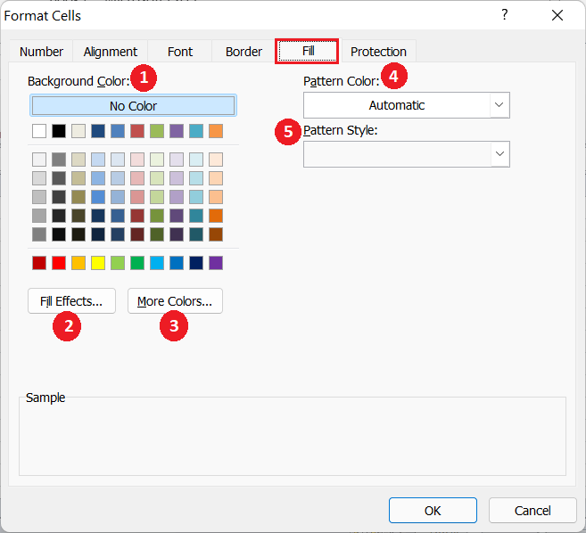
1. Background Color: Using the Background Color section, we can select the desired color to be applied as the cell’s background for the selected cells in the worksheet.
2. Fill Effects: Using the Fill Effects section, we can choose the color gradient or shading effect and the direction of effect.
3. More Colors: Using the More Colors section, we can create any custom color to be used as a cell’s background.
4. Pattern Color: Using the Pattern Colors section, we can add additional pattern color for the selected style of pattern used in the cell as shading or background.
5. Pattern Style: Using the Pattern Style section, we can choose between various predefined patterns to be used in addition to the cell background color.

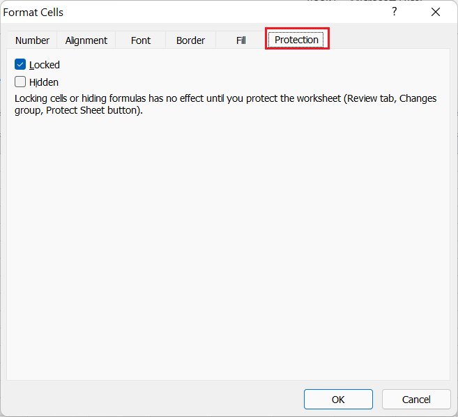
Protection tab

The Protection tab provides two specific options, namely Locked and Hidden. Both the options do not draw effect until we protect the worksheet. If we select the Locked option under the Protection tab, Excel restricts us to make the following changes in selected cells:

• Typing data into a blank cell.
• Changing cell data or formulas.
• Changing cell size.
• Moving the cell.
• Deleting a cell or its contents.

If we select the Hidden option under the Protection tab, Excel hides the formulas for corresponding cells from the formula bar. However, the results will be the same.

How to format a cell in Excel?

• First, we need to select the cells in the sheet.
• Next, we need to go to the Format Cells window and adjust the preferences from the respective tabs, such as the Number, Alignment, Font, Border, Fill, and Protection.
• After adjusting the preferences, we must click the Ok button to apply the changes in the sheet.

Important Points to Remember

• Conditional formatting is another powerful Excel tool that helps users format specific cells based on various conditions. However, it is not found under the Format Cells dialogue box. Instead, it is placed under the Home tab inside the Style group.
• Excel’s format painter tool helps users copy one cell’s formatting to another. It can be accessed from the Home tab inside the Clipboard group.
• Apart from the shortcut ‘Ctrl + 1’, we can also use the keyboard combination ‘Alt + H + FM’ to instantly launch the Format Cells dialogue box.

---