Formula for percentage of total in Excel
Percent calculation is a basic task to do in Excel. Every time the user wants to know how much work is done. It can be easily found by calculating the percentage of total of the work done till yet. This chapter is based upon calculating the formula for the percentage of total in Excel.

You will find the percentage calculation as an essential operation to do. To find the percentage of total for your data, you should know its formula. In this chapter, you will know the formula and learn how to calculate the percentage of total for data stored in an Excel sheet.
Basic formula to calculate the percentage
The basic formula to calculate the percentage that we generally use in mathematics is given below:
This formula can also be used in Excel to calculate the percentage. But the percentage and percentage of total are different terms. So, the formula for percentage of total is different.
Formula for the percentage of total
The percentage of total formula has a little bit of change than the percent formula. Below is the formula to calculate the percentage of total –
In this formula, part of the work done is divided by the total work but not multiplied by 100.
For example, A month expense is 3000 (cell A3) and the total expense is 24800 (cell B3). So, after applying the percentage of total formula, i.e., =A3/B3, it returns 12% after applying the percentage format on the resultant value.
Basic Introduction of percentage
Percentage is one of the essential formulas of mathematics that the Excel users may require to calculate the percentage on Excel data. Percentage is calculated using the basic operation (multiply and division) of mathematic, we described above.
People use the percentage calculation in their daily life. Fractions are converted to a percentage by multiplying them by 100%. Here, 100% is actually equal to 1.
Example to calculate the percentage of total
We have a list of travel expenses for a year (January to December) in column B. Here, we will calculate the percentage of expenses for each month. Before anything else, you need sum of expense (total expense) so that we can calculate the percentage of total.
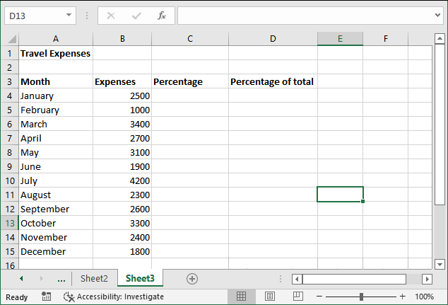
Step 1: Firstly, we will calculate the total of all months. For this, write the formula to find the total sum of the given months in the B16 cell.
=SUM(B4:B15)
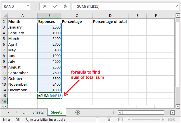
Step 2: Hit the Enter key and get the calculated sum, i.e., 31200.
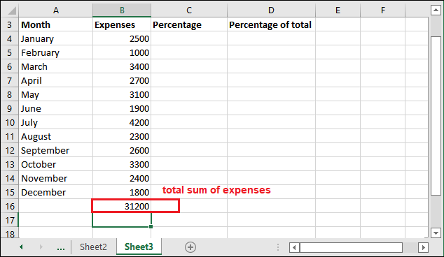
Now, calculate the simple percentage and percentage of total for the first month. In the column C, we will store the result of percentage and in column D, we will store the result of percentage of total.
Step 4: For the January month, use the following formula in which the January amount is divided by the total. This formula is for simple percentage calculation.
=(B4/B16)*100
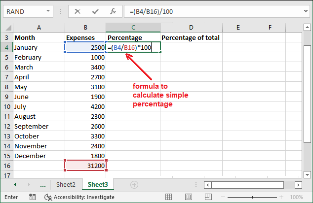
Step 5: Hit the Enter key and see the contribution of January month expenses from the month total. It is currently not in percent form.

Step 6: Now, use the following formula to find the percentage of total and see how it is different than the simple percentage.
=B4/B16
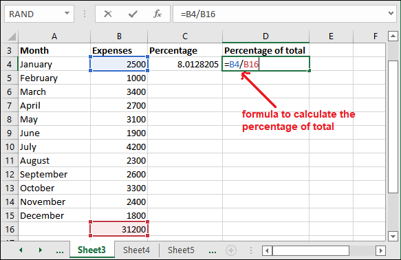
Step 7: Hit the Enter key and see the contribution of January month expenses from year total (percentage of total).

Currently, both resultant values are in decimal form rather than percent. We will later change it into a percentage after calculating for all other months.
Now, use the same formula with other month expenses to calculate the percentage. Or follow the below steps for fast calculation. We will autofill the formula for other month expenses (till row 15).
Make the denominator absolute
We want the denominator to be fixed for all percentage calculations so that each month expense will divide by the same total. So, we want to make the denominator an absolute reference. For this, make a little bit change in the formula by adding $ in the denominator row and column.
$ before the cell reference in formula will fix the value. After adding the $ to the formula, the formula will be something like below:
=(B4/$B$16)*100
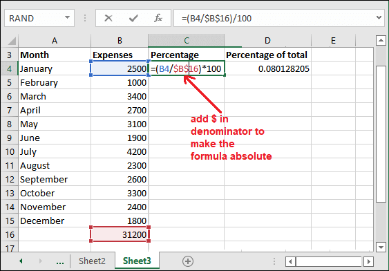
Here, $B indicates not to rewrite column and $16 to rows. The $ sign makes the value absolute. This one is the most important step. So, do not forget it even by mistake.
You will get the same result after making the percentage formula absolute. Now, make the percentage of total formula denominator too.
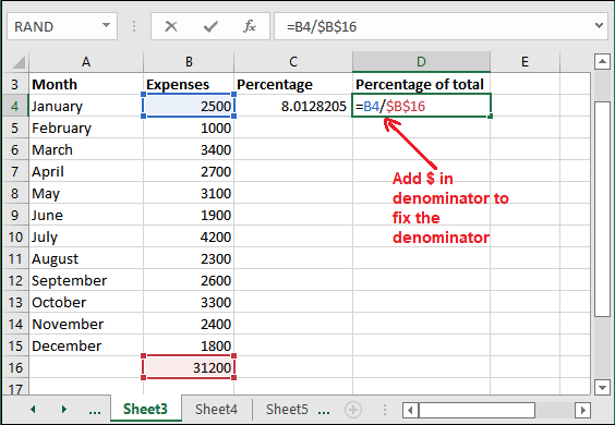
Now, the denominator is fixed for all the percent calculations.
Calculate percent for other months
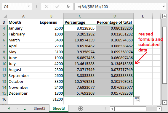
Now, we will find out the percent of total for other months. Select both the cells for simple percentage and percentage of total for January month (C4) and take the cursor at the bottom right corner of the cell.
Step 1: A plus (+) will appear. Drag this + sign below to cell C16. See that the percentage is calculated from January to December using a few simple steps.

Step 2: You will notice that the result is in received as a decimal value that is a long number. If you want to round off the value after two digits, you can do it easily in Excel.
Change decimal to percent (Percentage formatting)
We have calculated the percentage of total for all months, but it is currently in long decimal numbers. We want to show the calculated data as a percentage.
Follow a small click process to change the decimal to percentage:
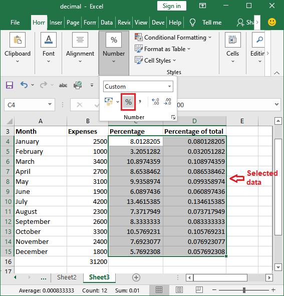
Step 1: Select all the calculated values in column C. Then, click the Percent Style (%) button inside the Home tab.
Step 2: See that all decimal values are converted to percentage format.
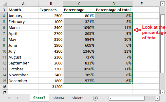
You can also increase and decrease the number of decimal values to be shown after the decimal point. For this, you can use the Increase Decimal and Decrease Decimal present on the ribbon. If you need, you can use it.
Along with the percent and percentage of total, you have seen the difference in both calculation results.
Example 2
It is an example of calculating the percentage of total for the student marks that they scored in different subjects. The maximum marks of each subject are 100. Here is an Excel sheet containing the marks of the 6 students.
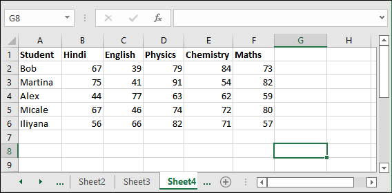
Follow the steps to find the percentage of total.
Step 1: First of all, calculate the total of marks for each student individually in a corresponding column by writing the following formula –
=SUM(B2:F2)
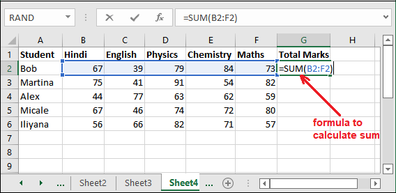
Step 2: Hit the Enter key to get the calculated sum for the first student.
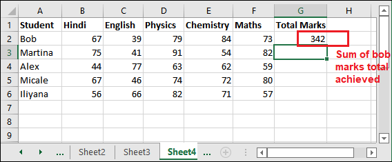
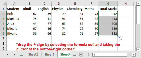
Apply the same formula to calculate the total sum of the marks for all students by changing the cell reference only or by dragging the G2 cell formula in the below cells.
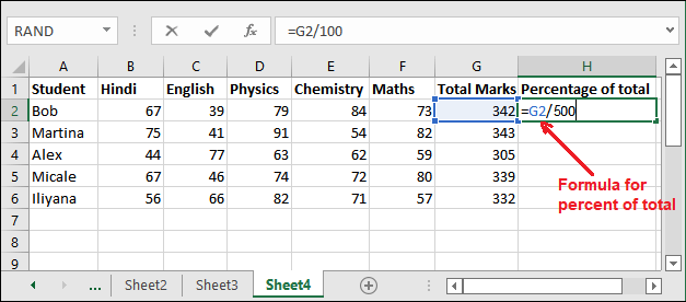
Step 3: Now, divide the calculated sum by the 500 (total of maximum mark for 5 subjects) and store the result in another cell. The formula will be –
= G2/500
Step 4: Hit the Enter key and get the result for the percentage of total.
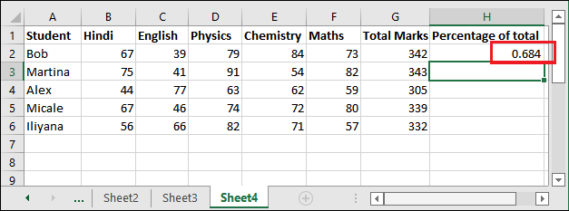
Step 5: Use the same formula for other cells and see the result in the end.
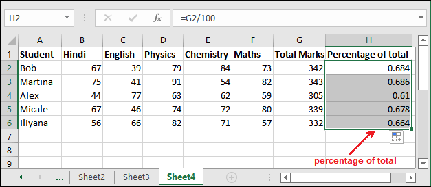
Apply the percentage formatting
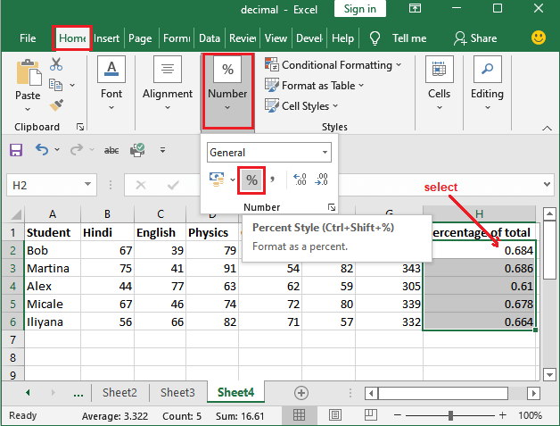
Step 5: To apply the percentage formatting, select all cells of the calculated percentage of total and click the Percentage (%) button inside the Number group in Home tab.
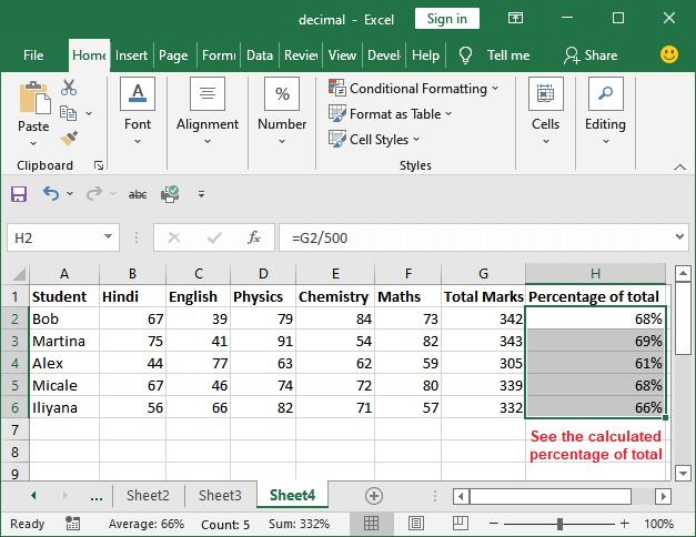
Step 6: See the final result for the percentage of total.
Example 3: Handle #DIV/0 Error
Following is an example of sales and target achieved by the number of employees. Some of the values in the sheet can be null too that can raise the #DIV/0 error. So, with the help of this, you will learn how Excel can handle this error.
We have the following set of data for this example, for which we will calculate the percentage of total.
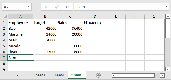
Follow the steps to find the percentage of total with some null values.
Step 1: Write the formula (=sales/target) in the D3 cell.
=C2/B2
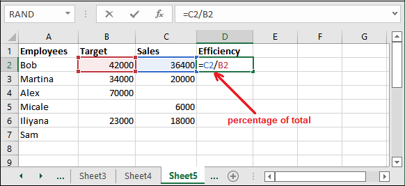
Step 2: Hit the Enter key and get the result calculated in the cell. Then, change the format of the resultant data by choosing the percentage format.
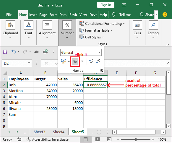
Note: To format the data from decimal to percentage, you need to select the targeted value and click the Percentage (%) sign inside the Home tab.
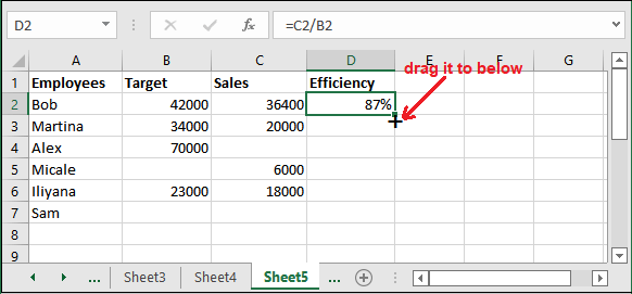
Step 3: See that the decimal result changed to percentage. Now, select the cell and drag the + sign below to copy the same formula for other corresponding data cells.
Step 5: See that – we got the result for all data. See, some of the results are fine but some are with #DIV/0! error. It is called percentage error.
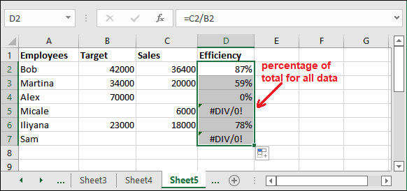
This error was for those calculated percentages whose either target (denominator) or target and sales both were null.
If you get the percentage error, you can remove it using the IFERROR function.
Step 6: To eliminate this error, make the change in the formula wherever you get the percentage error. For example, for D5 cell error result, the formula will be –
= IFERROR(C5/B5, 0)
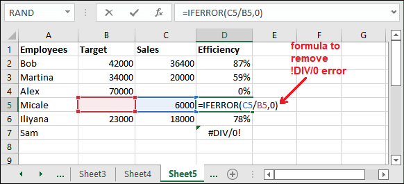
Step 7: Now, hit the Enter key and see the result of what it returns after using the IFERROR() function with the percentage of total formula.
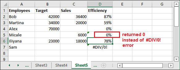
The #DIV/0! Error is replaced by 0. In the same way, you can use the IFERROR() function to remove the percentage error.
Key takeaway of percentage
- Percentage is a proportion per hundred.
- If you get the percent error, you can remove it using the IFERROR function.
- Percentage is calculated by dividing the numerator by denominator and then multiplying its result by 100.
- Usually, the users get the calculated percentage in decimal. The Excel users have to explicitly change it to percent form using % inside the Home > Number.
- Or the users can directly use the Ctrl+Shift+% shortcut command to change the data into percentage.
- Besides this, you will also see the Increase Decimal and Decrease Decimal to see the percentage in a proper way.
What is the percent change formula?
The formula for percent change is created by dividing the difference of new value and initial value by initial value. The formula will be like –
The percent change formula helps users find the percent increase and percent decrease between the two values. A positive percent indicates the percent increase, while a negative percent indicates the percent decrease.
Calculate percent change in Excel
The percent change formula is probably one of the most often used formulas in Excel that users use. The Excel formula for percentage change, or you would say percent increase and percent decrease.
For example¸ you can use the following formula for percent change if you want to calculate the percent change between A and B values.
Here, the values A and B should be correctly determined while applying the formula to Excel data. For example, yesterday, the price of the apple was 80, but now it is 100. It means apple price has been increased by 20, i.e., 25%. In the next scenario, if the apple price was 100 yesterday, but now it changed to 80. It means the price has been reduced by 20, i.e., 20% decrease.
If you consider the above formula for these values, the formula for percentage change will be as follows:
Now, let’s try to apply this formula on Excel data to see how this formula works in case of percent change.
Example 1: Percent change between 2 columns
Step 1: We have an Excel spreadsheet that contains the last month price of fruits in column B and current month price in column C.
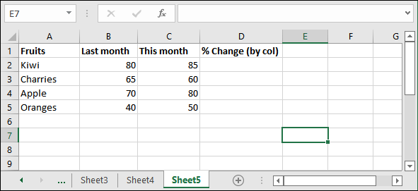
Step 2: Enter the following percent change formula in cell D2 to find the percentage change between new value and old value.
=(C2-B2)/B2
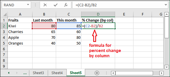
Step 3: Hit the Enter key and get the increased/decreased percentage for this month compared to the previous month.

Our data is already in percent style. If your data is in decimal style, select the resultant cell and click the Percent Style button to change the decimal result to percentage.
Step 5: Now, to copy the same formula in the other cells, just go to the previous resultant cell and take the cursor to the bottom right corner of it. You will see a + sign near it.

Step 6: You will now see the result for other cells by copying the formula of percent change.
This example for calculating the percent change between two columns.

Example 2: Percent change between rows
We calculated the percent change between two columns having prices for the last and current month in the previous example. This time, we have only one column. So, we will calculate the percent change between two rows.
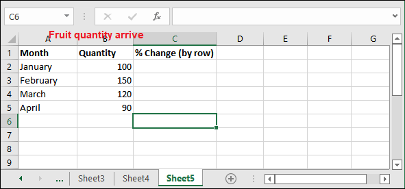
Step 1: Suppose that we have a column containing the weekly or monthly sales. Use the following formula to calculate the percent change between row data.
=(B3-B2)/B2
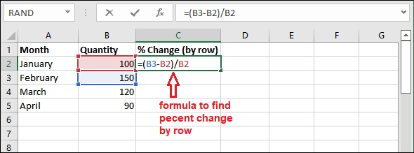
Here, you can take B2 as the old value and B3 as the new value.
Step 2: Now, press the Enter key on your keyboard and get the percent change result.
Our data is already in percent style. If your data is in decimal style, select the resultant cell and click the Percent Style button to change the decimal result to percentage.

Step 3: See the percentage change result of two rows in percentage style format.


