

Freeze panes in Excel
Excel has a freeze pane feature to freeze the part of the Excel worksheet. It is used to freeze the row and column. When the Excel worksheet is large, freeze pane is a useful option to freeze the particular part of the worksheet and make the other part scrollable.
In Excel, users can use the Freeze Panes feature of Excel to freeze the row or column of the worksheet. They can freeze panes to freeze the single or multiple rows/columns. Rows and Columns keep visible when they are frozen.
When to lock cells?
Whenever you work with the large worksheet with a lot of data, it is difficult to compare data. When you scroll the worksheet horizontally and vertically, the data of above cells hide with scrolling. In this type of scenario, Excel enables several methods, including Frozen Panes, New Window, and Split your worksheet.
Sometimes, you want some rows or columns always in your worksheet. Here, freeze panes feature help to lock the cells so that you can see the worksheet however you want. Freeze pane locks the specific row or column and makes them visible for the entire sheet scrolling.
Where is Freeze Panes option?
Sometimes, we need to scroll the entire worksheet and also want some row or column available through the entire worksheet scrolling. These particular rows or columns should not be hidden when you scroll the worksheet. In that case, Freezing the row/column will help you to freeze the data for the entire worksheet scrolling horizontally and vertically.
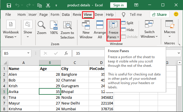
Freeze Panes is a feature of Excel that enables the users to lock the Excel rows and columns. This is available inside the View tab in the Excel ribbon. Inside the View tab, you will see a Windows group where this Freeze Panes option is present.
Method to freeze pane
Excel enables three methods to freeze the pane.
- Freeze Pane
- Freeze Top Row
- Freeze First Column
Properties of freeze pane
There are some points that you should be aware with them –
- Once the worksheet is frozen using the freeze pane feature, you cannot unfreeze the worksheet by undoing the action. You have to unfreeze it manually.
- If you freeze the top row, only the first row of the sheet will be frozen. You cannot freeze the column at the same time.
- Similar to Point No. 2, if you freeze the first column using Freeze First Column, only the first column of the worksheet will be frozen. You cannot freeze the row at the same time.
- If you apply the Freeze Pane option of Excel freeze pane feature, it can freeze the row and column simultaneously at the same time.
1. Freeze pane
When you freeze a part of the Excel worksheet using this freeze pane option, it keeps the rows and columns visible, scrolling is available through rest of the worksheet. This one allows the user to freeze the worksheet wherever he/she want. It freezes both rows and columns of the worksheet.
Example: Freeze the several rows and columns
In this example, we will freeze the first four rows and one column. For this, we will use the first option of the freeze pane that allows freezing the row and column at the same time.
Steps to freeze the pane
To freeze a particular part of the worksheet using freeze pane, execute the following steps –
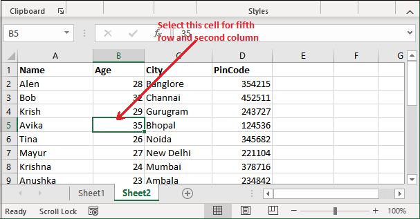
Step 1: Go to cell B5 for freezing the first four rows (4) and one column (A), then leave the cursor selection there.
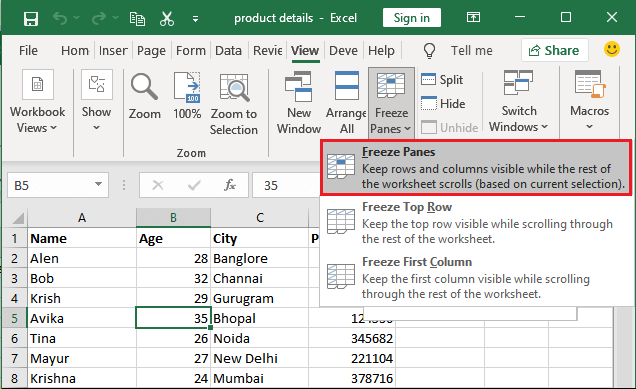
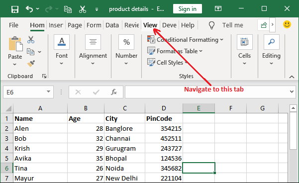
Step 2: Now, navigate to the View tab in the Excel ribbon, where you will see a Freeze Pane dropdown button inside the Window group.

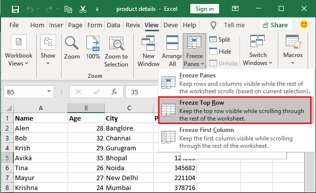
Step 3: Click on the Freeze Pane dropdown button and then click the Freeze Panes option to freeze the rows and columns.
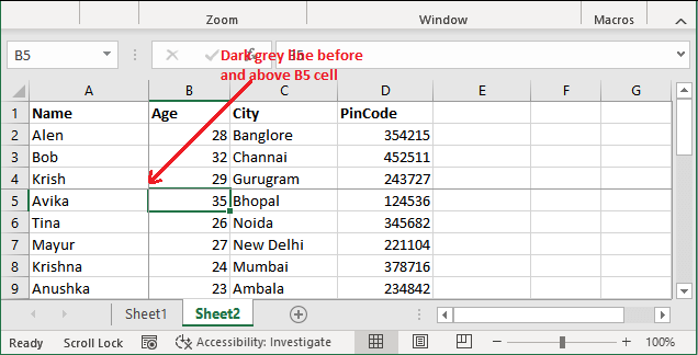
Step 4: Your first four rows and first column (till A4 cell) have been frozen successfully. Now, if you scroll the worksheet vertically or horizontally, till A4 row and columns are fixed and do not move with scrolling and rest of the worksheet will scroll.
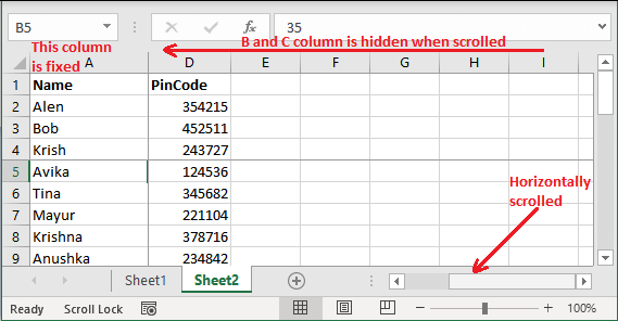
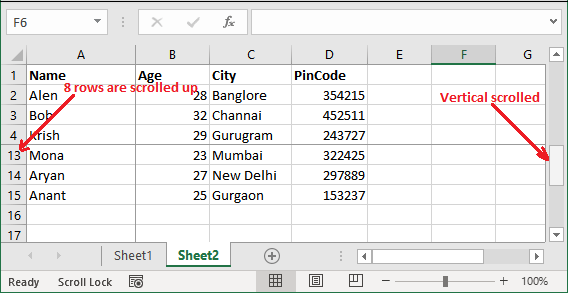
Horizontal Scrolling
See that the first column is fixed and does not hide while scrolling, whereas rest of the columns are scrolled left.
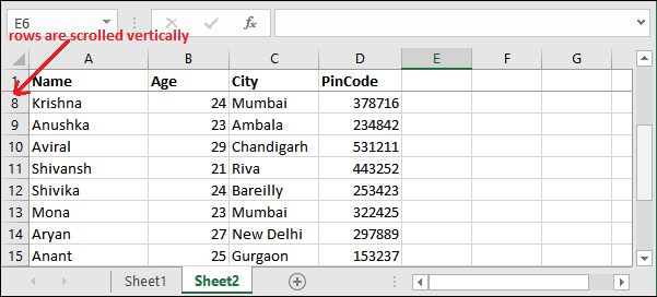
Vertical Scrolling
See that the first four rows are fixed and do not hide while scrolling, whereas rest of the rows are scrolled down.
Basically, this option allows to customize the freezing the number of rows and columns.
2. Freeze Top row
When you freeze the top row of your Excel worksheet using this freeze pane option, the first row of the Excel worksheet freezes and visible through the entire scrolling of the worksheet vertically.
Remember – in this method, only the first row is visible to the users after freezing through the entire worksheet scrolling. Steps are almost similar to the above method.
Steps to freeze the top row
In this example, we will freeze the first row (top row) of the worksheet. For this, Excel provides another option, i.e., Freeze Top Row. Choose this option inside the freeze pane and freeze the first/top row of the Excel worksheet. This will only freeze the row, not column.
To freeze only the first row of the worksheet and make it visible through the entire worksheet scrolling, execute the following steps –
Step 1: To freeze the first row, you do not need to select any particular cell. Navigate to the View tab of the Excel ribbon directly.
Step 2: Click on the Freeze Panes dropdown button and select/click the Freeze Top Row option here.
Step 3: The first row of the worksheet has been frozen and you can see that a dark grey color line has been placed below the first row.
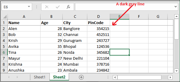
Step 4: Now, if you scroll up the worksheet rows vertically, the first row will keep visible and other rows will be scrolled.
3. Freeze First column
When you freeze the first column of your Excel worksheet using this freeze pane option, the first column freezes at its place and is visible through the entire scrolling of the worksheet horizontally.
After freezing the first column of the worksheet, this column is available through horizontal scrolling. Steps are almost the same as the Freeze top row method.
Steps to freeze the top column
In this example, we will freeze the first column of given Excel worksheet. For this, Excel provides another option, i.e., Freeze First Column. Choose this option inside the freeze pane and freeze the first column of the Excel worksheet. This will only freeze the first column, not rows.
To freeze the first column of the worksheet and make it visible through the entire worksheet horizontal scrolling, execute the following steps –
Step 1: To freeze the first column of the worksheet, you do not need to select any particular cell. Navigate to the View tab of the Excel ribbon directly.

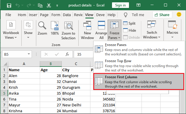
Step 2: Click on the Freeze Panes dropdown button and select/click the Freeze First Column option here.
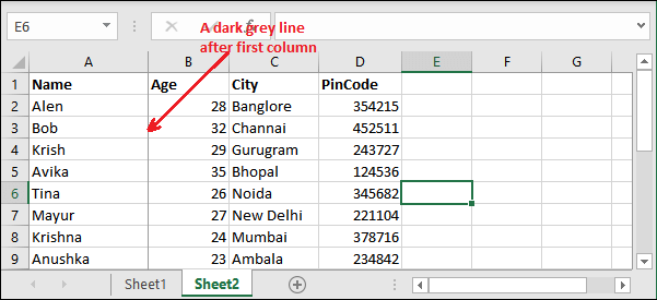
Step 3: The first column of the worksheet has been frozen and you can see that a dark grey color line has been placed after the first column.
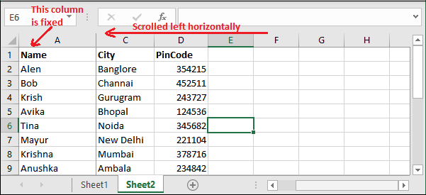
Step 4: Now, if you scroll up the worksheet rows vertically, the first column will keep visible and other columns will be scrolled.
When the user freezes the pane of the worksheet, a line is highlighted with dark grey color. Whatever freezing option you have chosen, you can get back unfroze it from the same option.
Unfreeze the worksheet
Once the worksheet row or column freezes using any option, you cannot undo the action. You can unfreeze it from the same View tab.
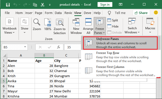
When the Excel worksheet is frozen, the first option under Frozen Panes is changed to Unfreeze Panes. From there, a worksheet can unfreeze. We will also show you the steps for this so that you can easily unfreeze the worksheet row/column.
Steps to unfreeze the worksheet
You can use the same steps for all whatever type you have chosen to freeze the worksheet row, column, or both. For example, topmost row is frozen of currently opened worksheet.
Following are the steps to unfreeze the worksheet –
Step 1: Navigate to the View tab and click the Freeze Panes dropdown button.
Step 2: Now, you will see the first option named Unfreeze Panes inside the dropdown list. Click this option to unfreeze the worksheet.
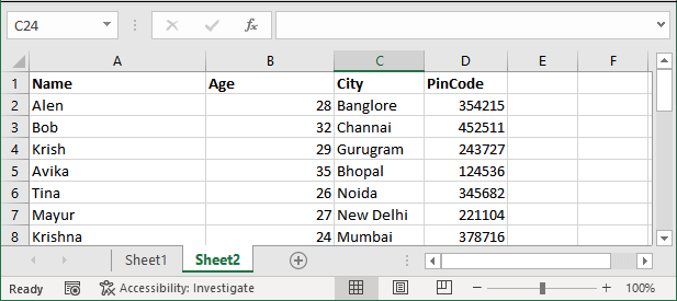
Step 3: You will now see that the grey line has been removed from the topmost row as the worksheet is unfrozen now.
Shortcut Key to freeze the worksheet
Excel has a shortcut key Alt+W+F to enable the freeze panes. After that, you can choose one of these three options:
- Press F key (alphabetic key) to freeze both row and column based on where your cursor is currently placed.
- Press R alphabetic key to freeze the top row of the Excel worksheet.
- Press C alphabetic key to freeze the first column of the Excell worksheet.


