How to Change Lowercase to Uppercase in Excel?

Unlike Microsoft Word, Microsoft Excel doesn’t have a Change Case button for changing capitalization. However, Microsoft Excel has three special functions that you can use to change the text’s case.

Functions are just built-in formulas that are designed to accomplish specific tasks. These three functions are UPPER, LOWER, and PROPER.

1. UPPER( ) Function

The upper() function allows you to convert all lowercase letters in a text string to uppercase.

For example, if you wanted to show cell B1 in an uppercase version of the text in A1cell, you could use the below function into B1.

2. LOWER( ) Function

The lower() function helps to exclude capital letters from text. You can take the value of any cell and converts it into lowercase text.

For example, if you wanted to show cell B1 in a lowercase version of the text in the A1 cell, you need to use the below function into B1.

3. PROPER( ) Function

The proper() function will evaluate text that is all proper case where each word starts with a capital letter and is followed by lower case letters. It converts the first letter of each word capitalized and leaves the other letters lowercase (Proper Case).

You can take the value of any cell and converts it into the proper case by using this function easily.

For example, if you wanted to show cell B1 in a proper case version of the text in A1cell, then you need to type the below function into B1.

NOTE: Once you created any of the above formulas, you can use the Excel Fill Handle to copy the function into as many cells as needed.

How to Use UPPER() Function

Follow the following steps to convert the lowercase text into an uppercase text in Excel. For example, you have the sales data collected according to each month.

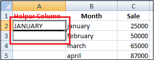
Step 1: Insert a new or helper column next to the one that contains the text you want to convert, as shown below.

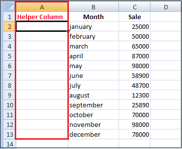
Step 2: Enter the formula in the adjacent cell of the A2 column.

B2 is the cell in the original column that has the text for conversion.

Step 3: Press the Enter.

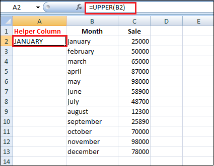
As you can see in the above image, cell A2 contains the uppercase version of the text from cell B2.

Step 4: Now, you need to copy the formula to other cells in the helper column.

• Select the cell that includes the formula.
• Move your mouse cursor to the small square or fill the handle in the lower-right corner of the selected cell until you see a small cross.
  
• Hold the mouse button and drag the formula down over the cells where you want it to apply.
• Release the mouse button.
  

Step 5: Now, you can remove the helper column.

So you have two columns with the same text data but in a different case. I suppose you’d like to leave only the correct one. Let’s copy the values from the helper column and then delete it.

• Highlight the cells that contain the formula and press Ctrl + C to copy them.
• Right-click on the first cell in the original column.

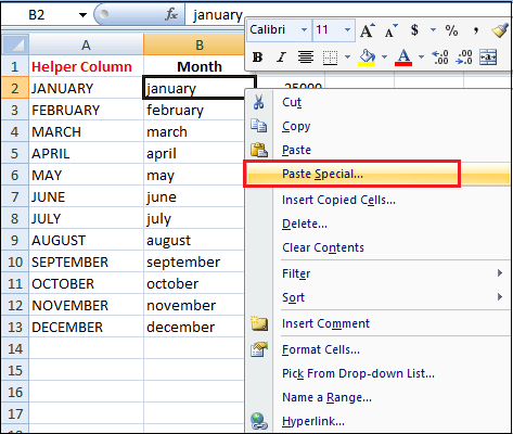
• Click on the Paste special in the context menu.
• And select the values from the options.
• Click on the ok

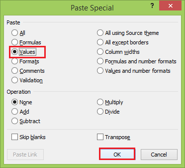
You need to pick only the text values option from the Paste Special dialogue box to avoid formula errors later.

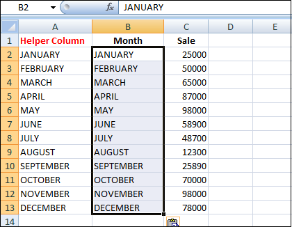
Step 6: Right-click the selected helper column and choose the Delete option from the menu.

Step 7: Pick the Entire column in the Delete dialogue box and click on the ok button.

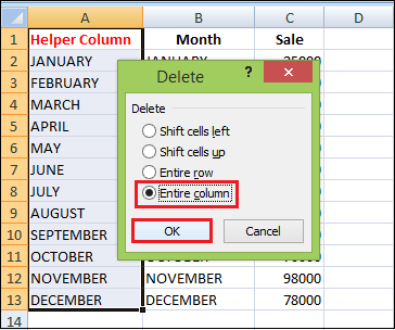
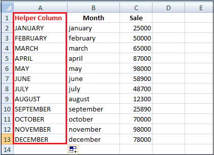
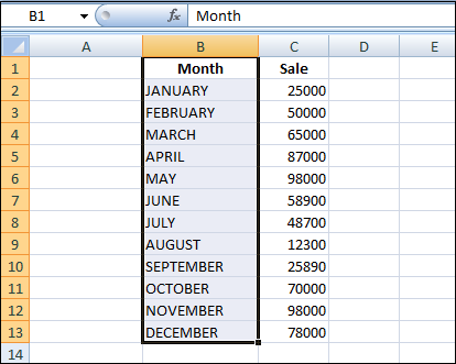
As a result, the excel sheet provides month column values in uppercase and looks like below.

Use Microsoft Word to Change Case in Excel

If you don’t want to use the Excel formulas, you can use special command for changing text case in word. Below are the following steps, which tell how this method works.

Step 1: Select the range where you want to change the case in Excel.

Step 2: Press Ctrl + C or right-click on the selection and choose the Copy option from the context menu.

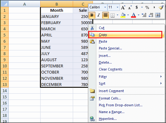
Step 3: Open a new Word document.

Step 4: Press Ctrl + V or right-click on the blank page and select the Paste option from the context menu.

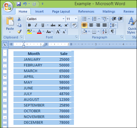
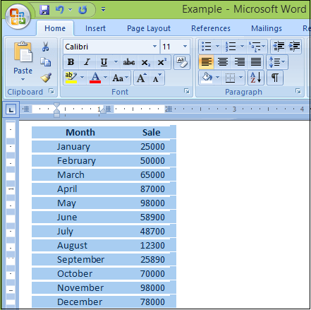
Step 5: Now, you’ve got your Excel table in word.

Step 6: Highlight the text in your table where you want to change the case.

Step 7: Move to the Font group on the Home tab and click on the Change Case icon.

Step 8: Pick one from five case options from the drop-down list.

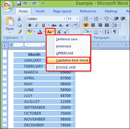
You can also select your text and press Shift + F3 until the style you want is applied. Using the keyboard shortcut, you can choose only the upper, lower, or sentence case.

Step 9: Now, you have your table with the text case converted in word. Just copy and paste it back to Excel.

Change Case with the Cell Cleaner add-in

Looking at all methods described above, you might still think that there is no easy way to change case in Excel. Let’s see what the Cell Cleaner add-in can do to change the case. Follow the following steps to apply this method:

Step 1: Download the add-in and install it on your system.

Step 2: After the installation, the new Ablebits Data tab appears in Excel.

Step 3: Select the cells where you want to change the text case.

Step 4: Click on the Change Case icon in the Clean group on the Ablebits Data tab. The Change case pane displays to the left of your worksheet.

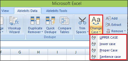
Step 5: Select the case you need from the list.

Step 6: Press the Change case button to see the result.

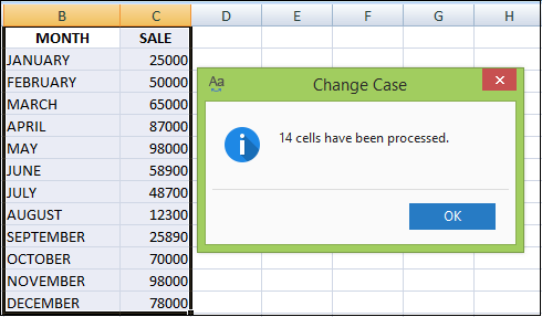
With Cell Cleaner for Excel, the changing case routine seems much more comfortable than other methods.

Besides changing text case, Cell Cleaner can help you to convert numbers in the text format to the number format, delete unwanted characters and excess spaces in your Excel table.

How to Change Case with Macro

You can also use a VBA macro for changing case in Excel 2010 and 2013. Below are three simple macros that make Excel convert text to uppercase, proper or lowercase, such as:

1. If you want to convert text into uppercase, you can use the following Excel VBA macro.

2. If you want to change uppercase into lowercase data, then you need to insert the code shown below into the Module

3. If you want to convert your text values to proper or title case, you need to use the following macro.