How to compare two columns in Excel?
When two or more columns contain complex data, which cannot be compared by just seeing them, Excel provides some predefined function for this.
Excel allows the users to compare the two column’s values. It can be done in several ways using different methods, such as IF, MATCH, and ISERROR functions. The method whichever you use will depend on the data structure and what you want from it. Either we can compare two or more columns in one go or one row at a time.
For example,
- Compare two column’s data row by row and get the result as either true or false.
- Compare two columns and highlight all the matching data points (available in both columns) in both columns. Conversely, highlight the differences (unmatched data points) in both columns.
Excel offers various methods and techniques of comparison. In this chapter, we will cover all necessary points that require to know for comparing two columns. Here, we are going to discuss the following topics in this chapter:
- Compare two columns by Exact row match
- Row by row comparison (simple comparison)
- Row by row comparison using IF formula
- Highlight matching rows
- Compare two columns and highlight the matches
- Compare columns and highlight matches
- Compare columns and highlights mismatches
Usually, when we have a large dataset with complex values, and we want to find out match and unmatched data. These methods of comparison help the users to get the expected result using these methods.
Compare two columns by Exact row match
It is the simplest way of comparison. It is a row-by-row comparison of data for two or more columns. We can get exact row matches for comparing two columns using three different methods, i.e.,
Method 1: Row by row comparison (simple comparison)
Method 2: Row by row comparison using IF formula
Method 3: Highlight matching rows
These methods of comparison are only used for row-by-row comparison of two or more columns. It is helpful when you want to find the match only in the same row, not in the entire dataset.
Usually, comparing two columns row by row is not a good idea when you want to find all the values having more than two matches in the whole selected columns instead of in the same row.
Features
- You can compare each row value of both columns one by one and get the result as either TRUE or FALSE.
- All values of both columns cannot be compared in one go using these methods. Therefore, it takes time to compare all rows of two columns.
Method 1: Row by Row comparison
This method is used for comparing two cells of the same row. It is a simple comparison. It means that we can compare two column’s data row by row without using any typical formula. For example –
The following is formula for comparing the first row of two columns, A and B.
We will just compare two columns row by row.
Return Value
It will return TRUE if both cells have exactly the same values. Otherwise, it will return FALSE as a result. The returned value stores in another column selected by the user while comparison.
Example
Now, see the example of how the comparison actually takes place.
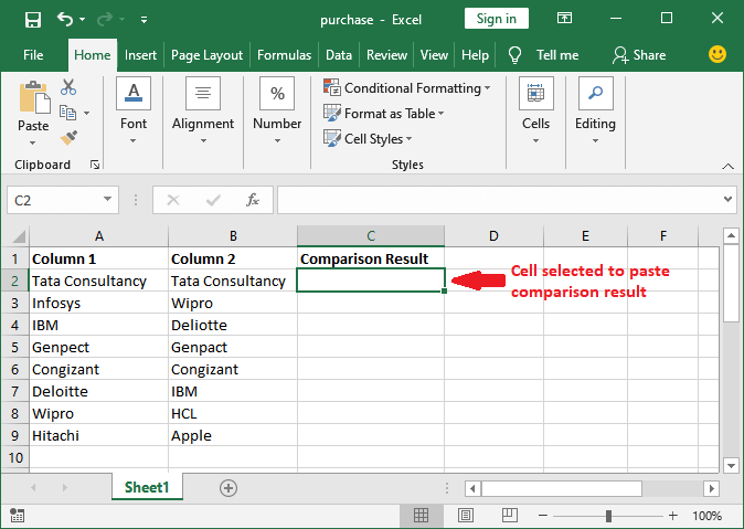
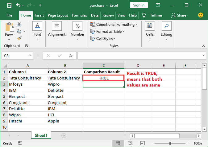
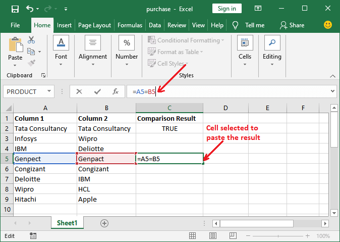
Step 1: Open an Excel sheet and select a cell where you want to paste the comparison result.
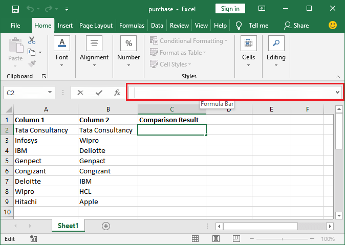
Step 2: Now, go to the formula bar, where you can write the formulas.
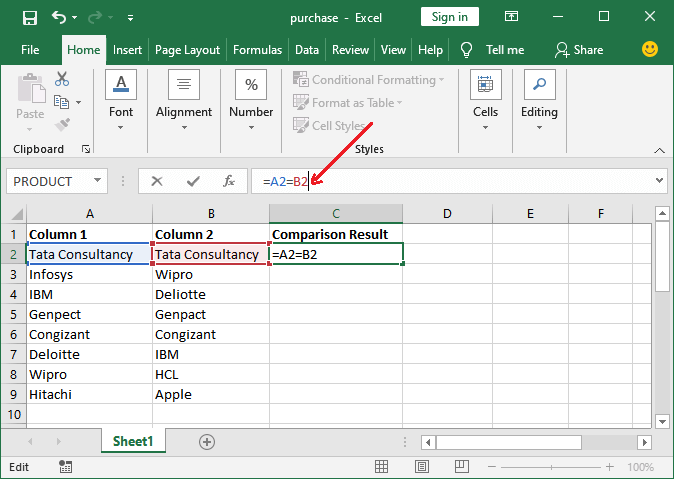
Step 3: Type the formula to compare the column row-by-row. E.g.,
=A2=B2 for comparing the second row of columns A and B and “press the Enter key“.
Step 4: You will get the result either TRUE or FALSE. See that it returned TRUE as both strings are exactly the same.
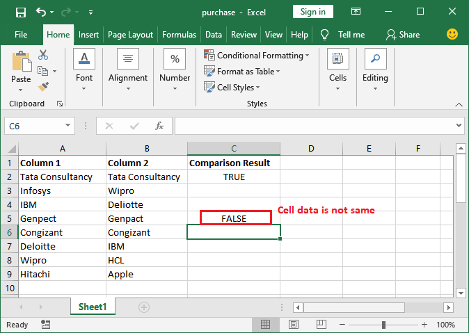
Step 5: Now, we will show you one for the FALSE result when values are mismatched. We will check the 5th row. So, type the following formula:
=A5=B5 and press the Enter key.
Step 6: See that it returned FALSE, which means that A5 and B5 are not the same. There is no change in both spellings.
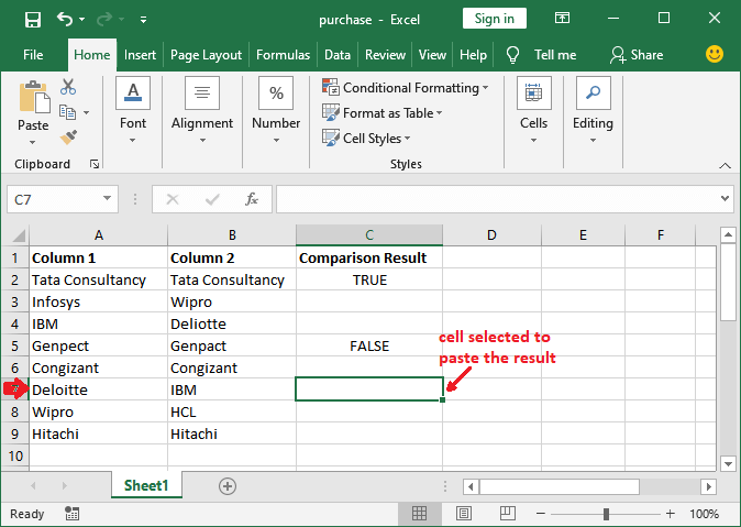
Similarly, you can perform more comparisons for other rows.
Method 2: Row by Row comparison using IF formula
This method is another way to compare two columns. It is almost similar to the above method. In this method, we will use the IF formula to compare two column’s data row by row using. For example –
The following is a formula for comparing the first row of two columns (A and B) using the IF formula.
This time it will return Match if both column’s values are the same, but if the exact match is not found, it will return Mismatch as a resultant value.
Note: You can also customize the result string in formula according to you whatever you want.
Return Value
It returns the first string if both cells contain exactly same data. Otherwise, it returns the second string that you have passed inside the IF function.
Example
Now, see the example of how the comparison actually takes place.
Step 1: Open an Excel sheet and select a cell where you want to paste the comparison result.
Step 2: Now, go to the formula bar, where write the formula to compare the column row-by-row for the 7th row. E.g.,
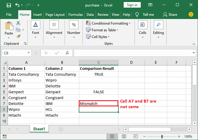
=IF(A7=B7, “Match”, “Mismatch”) and “press the Enter key”.
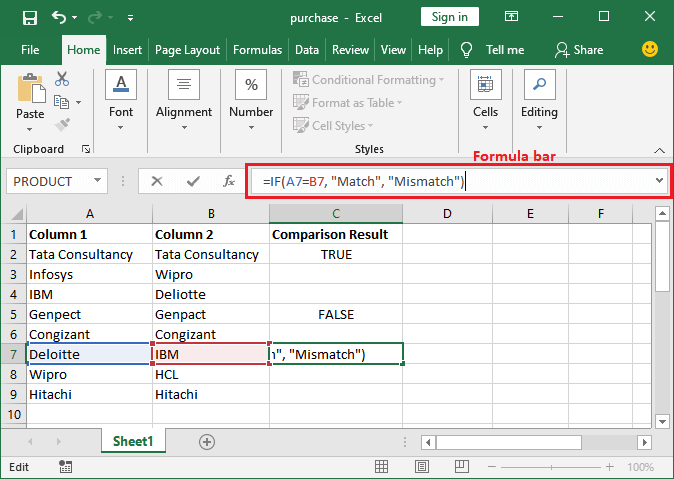
Step 3: You will get the result either Match if the values are same or Mismatch if not. See that it returned Mismatch as both strings are not the same.
Step 4: Similarly, check one more row data to get the match result. We will check the 9th row using the following formula:
=IF(A9=B9, “Match”, “Mismatch”) and press the Enter key.
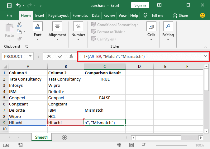
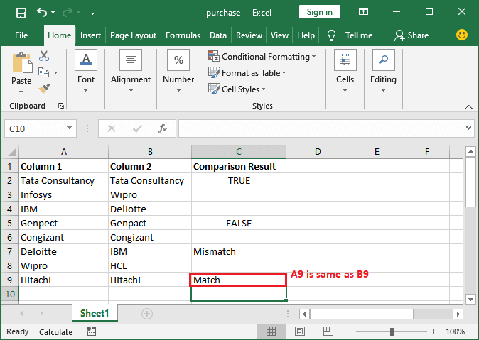
Step 5: See that it returned Match as the result, which means that A9 and B9 are same.
Similarly, you can perform more comparisons for other row’s data.
Method 3: Highlight matching rows
It is a bit different method than the above two one. Using this method, we highlight the row which has the same data in both columns. Conditional formatting is used for this method. It does not return any resultant string; it highlights the matches data row instead of returning TRUE or FALSE.
Note: You have to do comparison one-by-one for each row. You cannot check multiple rows data at once.
It is a useful method for comparing multiple rows in one go, by highlighting the matched data rather than getting the result in the third column. It saves the time of users by comparing and showing the result at once.
Result
The row will get highlighted if found the exact match in both column’s cells. Otherwise, the row will not be highlighted if match is not found.
Example
Let’s take an example to step by step comparison.
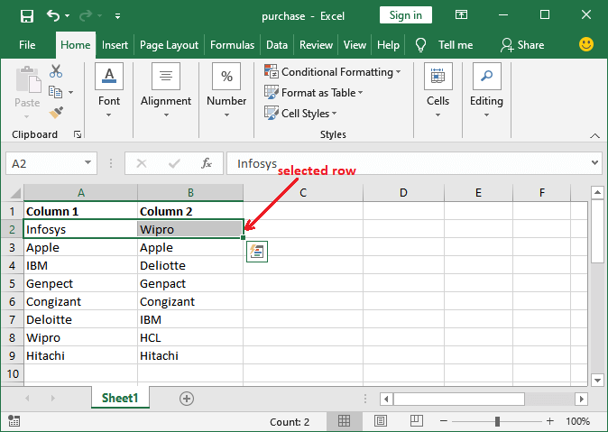
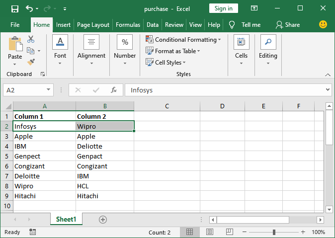
Step 1: Open your targeted Excel file and select the row you want to check whether the values are the same or not.
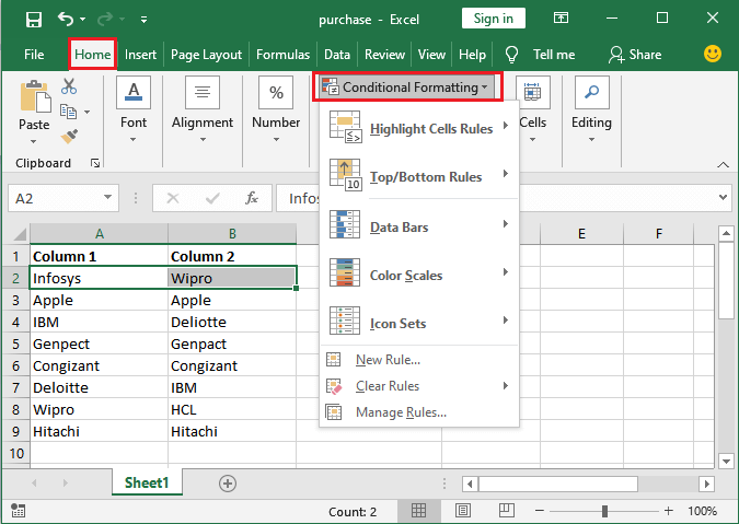
Step 2: In the Home tab, you will see an option named Conditional Formatting under the Style group. Click on this dropdown list.
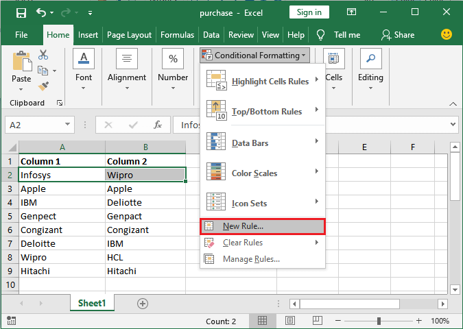
Step 3: From the dropdown list, click on the New Rule that will open a panel to set new formatting rules.
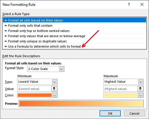
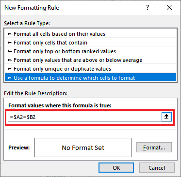
Step 4: Here, click on the Use a formula to determine which cell to format from the rule type list.
Step 5: Here, inside the formula field, specify the cells you want to compare in the following format, e.g., =$A2=$B2. This formula is for the second row.
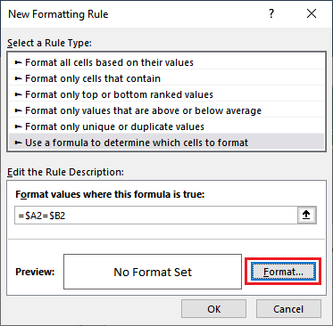
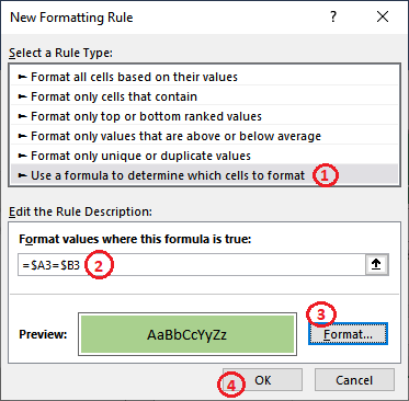
Step 6: In the end, specify the format for matched cell by clicking on the Format button and see the preview of it inside the Preview box.
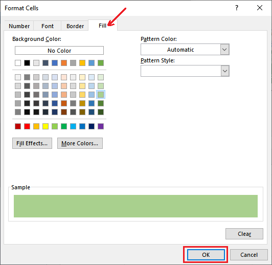
Step 7: Here, navigate to the Fill tab and choose a background color to highlight the matches and click the OK button.
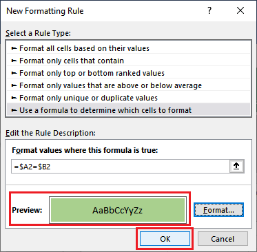
Step 8: See the preview inside the preview section and see how row will look like if match is found. After finalizing all the things, click the OK button to save the changes.
Step 9: You will see that the selected row has not been highlighted because the A2 and B2 cells do not contain the same values.
Step 10: By following the same steps, compare the next row data. See that everything is set up successfully. Now, click the OK button to get the result.
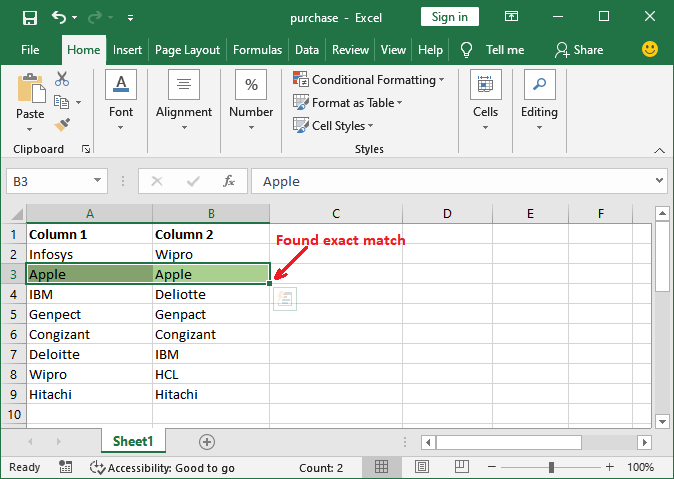
Step 11: Look at the following screenshot, that the 3rd row has been highlighted because it gets the same data in both columns.
Step 12: Similarly, we will check for all rows one-by-by.
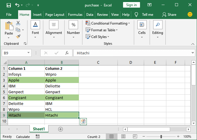
After comparing all the rows in both columns, see our Excel worksheet; that row having the same data in both columns has been highlighted, and remains are as they are.
It will highlight all the matching data row in the format you have chosen previously.
Compare two columns and highlight the matches
This method of comparison is also done using conditional formatting. It is a useful method to compare one column data with another column values and gets the matches highlighted after comparison.
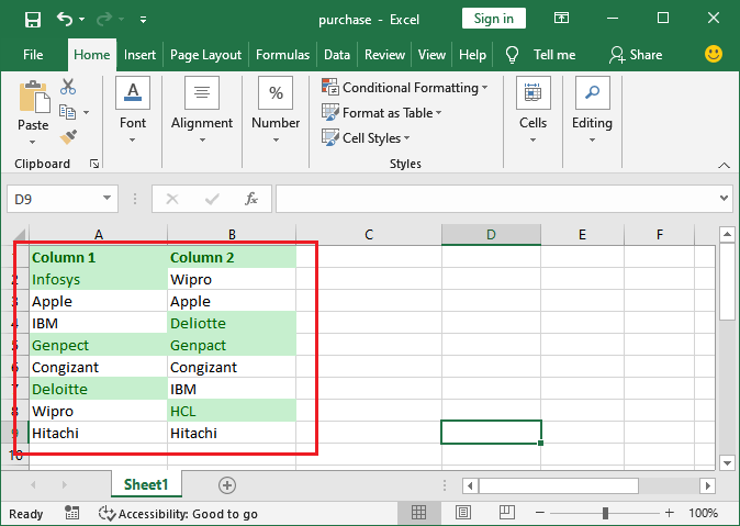
It is used to find the matches not only in the same row of the selected columns but in the entire selected dataset. Using this method, we highlight the cells data having at least two or more than two matches. For example –
Often, there are matches available but not in the same row. In this scenario, these methods of comparison help the users to find the matches. Something as is showing in the below screenshot:
Features
- All values of both columns are compared in one go.
- It saves the time of users by comparing the entire column with another column at once.
- You can either highlight all the unique or duplicate values, whichever you want.
There are two ways to compare columns and show their result, i.e.,
Method 1: Compare columns and highlight matches
Method 2: Compare columns and highlights mismatches
Compare columns and highlight matches
This method of comparison is not same as the row-by-row comparison. It works differently. In this method, we use duplicate functionality in conditional formatting. It means that the duplicate values will get highlighted after a successful comparison.
Following are the steps for comparing two columns and highlighting the matches:
Steps for column comparison
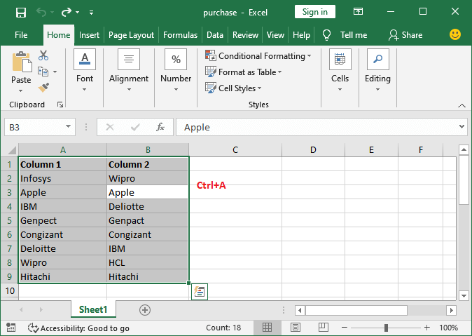
Step 1: Open your targeted Excel file. This time select all data using the select all Ctrl+A shortcut key in which you want to find duplicate values.

You can also select only two columns.
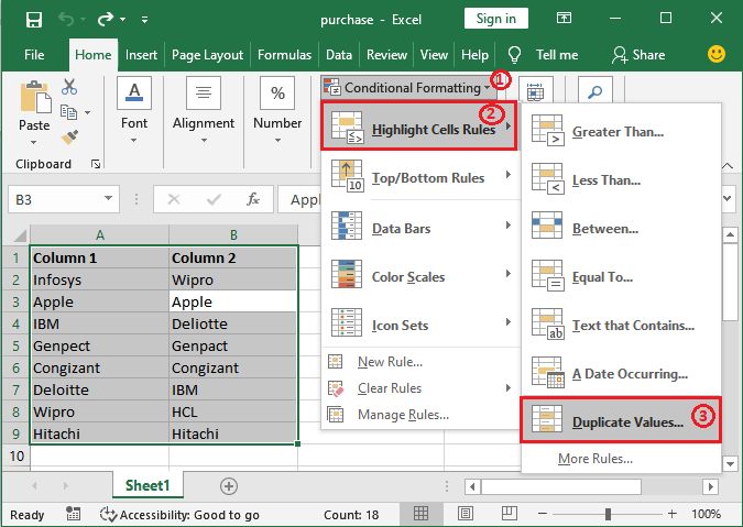
Step 2: In the Home tab, you will see an option of Conditional Formatting under the Style group. Click on this dropdown list.
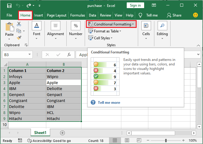
Step 3: In the dropdown list, hover the mouse to the Highlight Cell Rules option to expand more options and then click on the Duplicate Values.

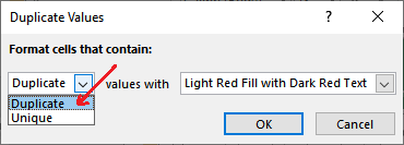
Step 4: Now, in the Duplicate Values dialogue box, ensure the Duplicate is selected in the given dropdown list. If not, select Duplicate here.
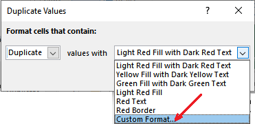
Step 5: Next, specify the formatting color for highlighting the duplicate values present in the selected dataset and click the OK button.

You can also customize the color and font other than the given ones. This means that you can set your format to highlight the duplicate values from the Custom Format.
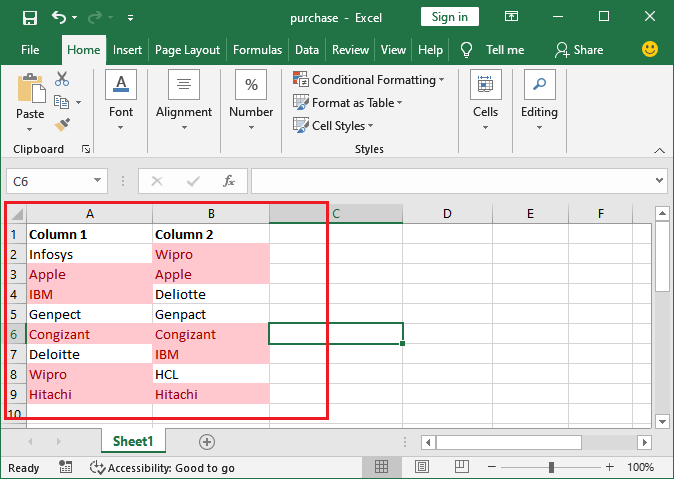
Step 6: See the below screenshot that all the duplicate values have been highlighted with red color. This comparison is for the entire selected data instead of row-by-row.
Compare columns and highlight mismatches
This method is almost same as the above one, but the difference is that – in this method, we highlight mismatches instead of matches. Thus, it works the same but resultant differently.
In this method, we use duplicate functionality in conditional formatting and highlight the values which are not duplicates in selected columns. It’s steps are almost the same as the above one. Follow the steps below to see how could it be done:
Steps for column comparison
In this example, we will use the same excel worksheet with the same content in it. But this time, we will highlight unique values present in this Excel worksheet.
Step 1: Open your targeted Excel file and select all data of it using the select all Ctrl+A shortcut key. You can also select only two columns.
Step 2: In the Home tab, you will see an option of Conditional Formatting under the Style group. Click on this dropdown list.

Step 3: In the dropdown list, hover the mouse to the Highlight Cell Rules option to expand more options and then click on the Duplicate Values.
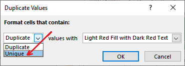
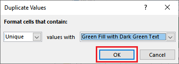
Step 4: This time, choose Unique from the dropdown to highlight the unique values instead of duplicate ones.
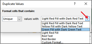
Step 5: Choose a format to highlight the unique values present in the selected dataset.
Step 6: Setup the format accordingly and then click on the OK button here.
Step 7: You can see that all the values, which are unique (only one in the selected dataset), have been highlighted. All values are highlighted in one go.