How to delete rows in Excel?

Deleting rows or columns in an Excel sheet is a very basic but useful operation of Excel. While working with Excel workbooks, the users may need to delete one or more rows of an Excel sheet. These rows can be blank or rows with data. Insertion and deletion of rows is common operations of MS Excel.

Delete the unnecessary rows to organize the worksheet. Excel enables various ways to delete one or more rows in Excel. It also offers shortcut keys for these operations, which can be used for quick operations. This chapter will have the methods of deletion of rows.

Why to delete rows?

Sometimes, the users do not require some rows longer. They want to delete the unwanted rows from the Excel sheet. For this, Excel offers quick and fast methods to delete the rows.

Rather than deleting the data of a row from the cell one by one, delete the entire row and make the process fast. The other rows will automatically get organized and shift/take the place of deleted row. The Excel users need to delete rows when they don’t need the data of the row anymore. Remember, it can also be a blank row.

There are a lot of methods to delete the unwanted rows (either blank or with data) and all are very easy and fast.

Delete a single row

By taking some steps, we will delete a single row in an Excel sheet. This row will contain some data. To delete a single row in an Excel sheet, follow the given steps below:

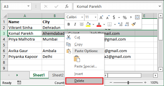
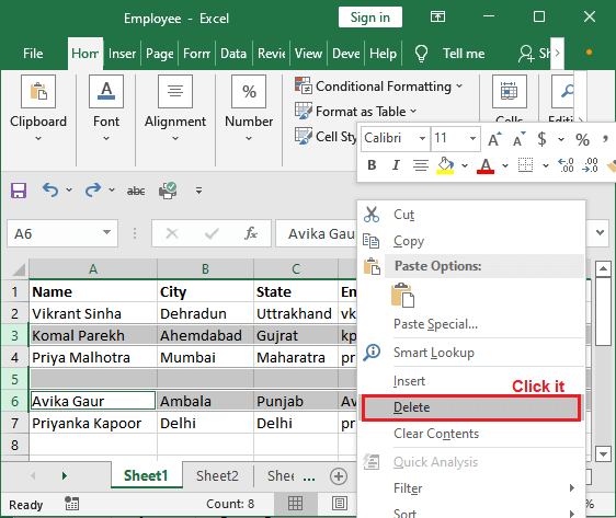
Step 1: Select the row you want to delete from the row header present at the left side of the worksheet. E.g., we have selected row3 for employee Komal Parekh record.

Step 2: Right-click on it and select Delete.

Step 3: You will now see that the row3 (Komal Parekh) record has been successfully deleted and the rows below it shifted to above.

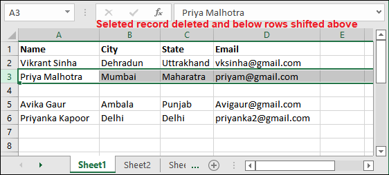
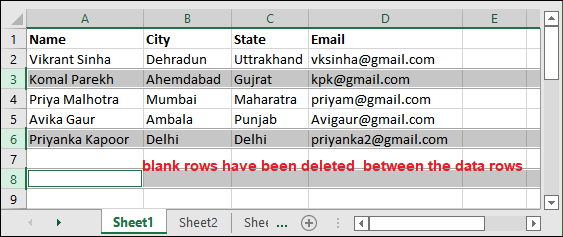
Same as the user can delete any blank row between the data.

Delete multiple rows

By taking the help of some steps, you will learn to delete multiple rows in an Excel sheet. We undo the changes of the previous example and use the same data for this example. This row will contain some data. To delete multiple rows in an Excel sheet, follow the given steps below:

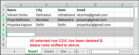
Step 1: Select all the targeted rows you want to delete from the row header present at the left side of the worksheet by taking the help of Ctrl key.

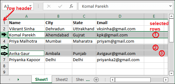
Step 2: Right-click one of the selected rows and click Delete from here.

Step 3: You will now see that all the selected rows (including blank row) have been successfully deleted and the rows below it shifted to above.

Delete blank rows manually

Blank rows between the data are very annoying sometimes and you want to delete them. The Excel users can delete the blank rows by finding them manually. This method is as simple as you followed the above one.

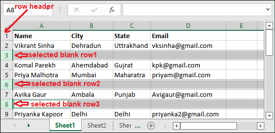
For example, we have the data with some blank rows in between. Now, the point is we want to delete these unwanted blank rows.

Step 1: Select the blank row from the row header by holding the Ctrl key.

Step 2: Right-click one of the selected rows and choose Delete.

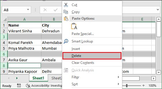
Step 3: You see that all the selected blank rows have been deleted.

There is a shortcut key Ctrl- using which you can delete the selected row or column.

This method is good and short when you have limited data in which blank rows are easy to find. But when you have a lot of data in a single sheet, it becomes difficult to find the blank rows inside them and time taking too. So, we have another solution for it.

Delete blank rows using Go To Special

Blank rows between the data are very annoying sometimes and you want to delete them. It will be hectic to find each blank row and delete it one by one. Rather than doing this process, Excel enables other ways to delete the blank rows at once.

Go To Special is a feature of Excel that will select the blank rows for us. By taking an example for it let us see how it works. We will illustrate the steps as follows:

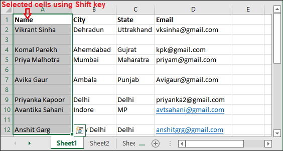
Step 1: Select a column in an Excel sheet, including blank rows. For this, select first cell A1 and hold the Shift key, then select the last data cell, i.e., A12.

Step 2: Inside the Home tab, click the Find & Select (in Editing group at the end of the Excel menu) and choose Go to Special command from the list.

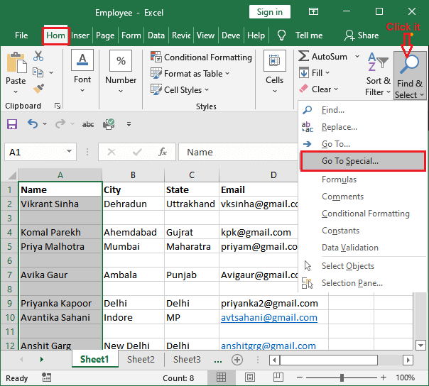
“Go To Special command will help us to select only blank rows in the selected column data.” You can also select the Go To command and then move to the Go To Special.

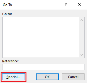
If you mistakenly opened Go To dialogue box, click the Special button to switch on the Go To Special panel.

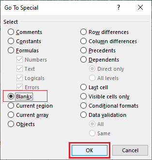
Step 3: On the Go To Special panel, mark the Blanks radio button and then click OK.

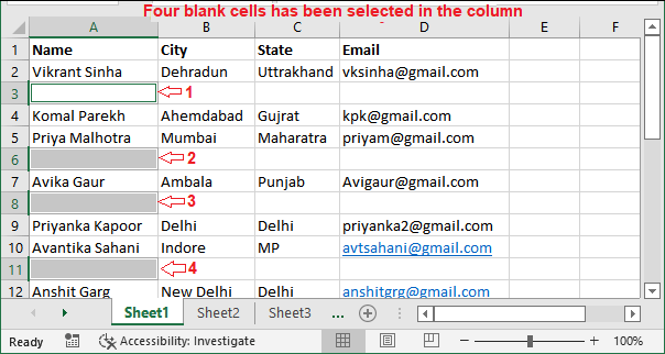
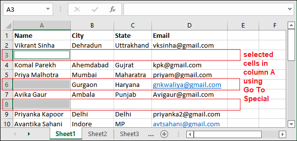
Step 4: All the blank cells in the selected column (Column A) have been selected. Note that only cell is selected rather than the entire row.

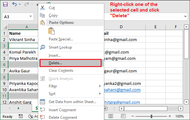
Step 4: Now, we will delete the blank rows on the basis of selected blank cell of the column. For this, right-click any of the selected cells and click the Delete command.

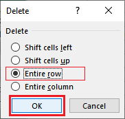
Step 5: Here, select the Delete Entire Row option and click OK.

Step 6: See that all the blank rows have been deleted based on the selected blank cells.

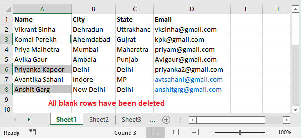
Like this, an Excel user can find thousand of blank rows in an Excel sheet and delete them using a very short process. This is good when you have too many blank rows scattered in the entire sheet.

Disadvantage of using Go To Special method

You have seen that the Go To Special feature is one of the best ways to find and delete the blank rows in an Excel sheet. But it also has disadvantages too, i.e., it deletes the entire row based on a single blank cell returned from the Go To method.

Let us understand this with a scenario:

For example, It might be possible that the selected cell using Go To Special may have the data in their corresponding row. As you delete the entire row for the selected blank cells, data will get deleted.

Selected all blank cells in column A using Go To Special method.

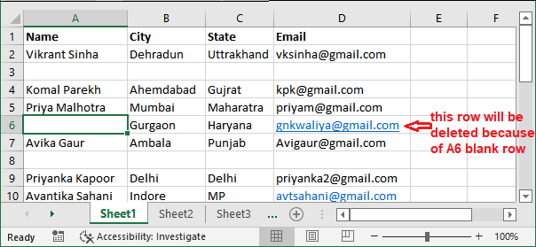
Now, on deleting the entire rows corresponding to the selected blank cells. The output will be like, as given below:

See that row 6 has also been deleted along with the as Go To Special found A6 as a blank cell. It was the biggest disadvantage of this method.

We have another solution for this offered by MS Excel, i.e., filter method.

Delete blank rows using Filter

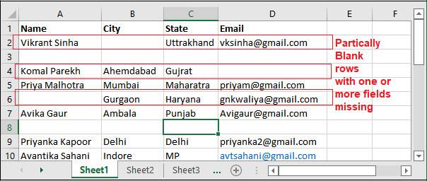
Another way to delete the blank rows is filter that does not delete the entire row based on a single blank cell (get from Go To Special). It will not delete the entire row based on a single blank cell. We have designed a dataset in an Excel sheet where some cells are not completely blank.

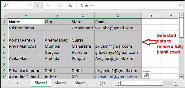
Initially, we have the following dataset in which some rows are semi-blanked. Here, rows 2, 4, and 6 are partially blank and rows 3, 8 are completely blank.

Step 1: Select the targeted dataset from which you want to delete the completely blank rows between the data.

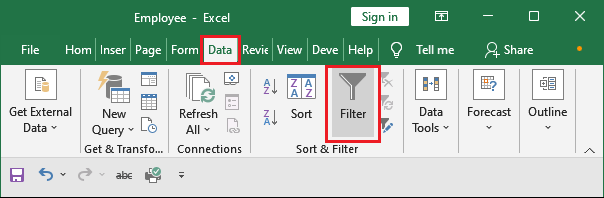
Step 2: To highlight the column header, just go to the Data tab and click the Filter button inside Sort & Filter.

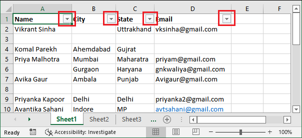
Step 3: You see that a dropdown button is placed next to each column header. It will allow filtering of the blank rows.

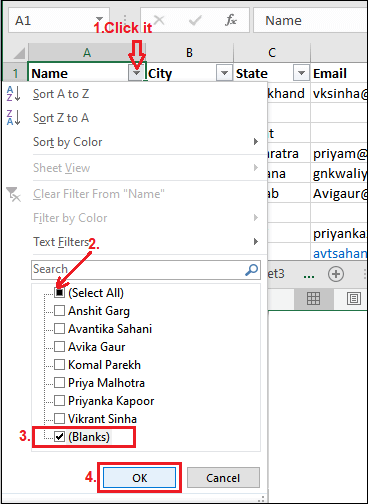
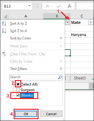
Step 4: Click the dropdown button next to column A to filter the blank rows in this column. Here, uncheck the Select All checkbox and then select the Blanks checkbox.

Click OK.

Step 5: See that the sheet data has been filter based on the blank rows in column A. Fully blanked rows are represented in the row header by blue highlighted row number.

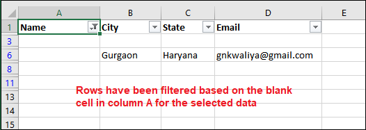
Here, one partially blank row has remained.

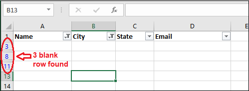
Step 6: Now, use another column (column B) to filter the remaining data in the sheet.

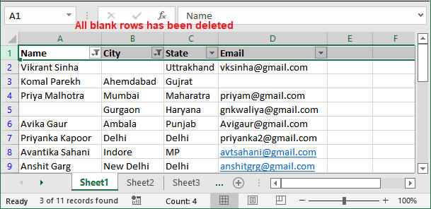
Step 7: No row remained with data. All the blank rows are shown by blue highlighted color in the row header. After filter, three blank rows are found.

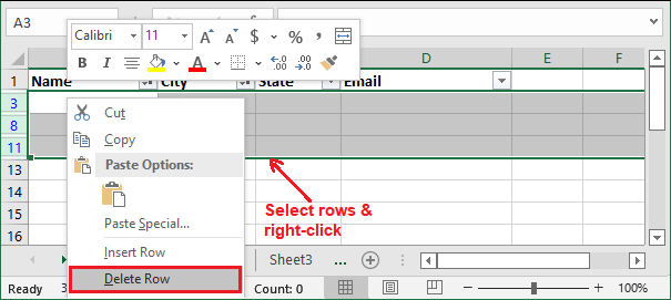
Step 8: Now, Select these rows and right-click on them. Click the Delete Row option.

Step 9: This time, only fully blank rows have been deleted rather than partially blank rows. The output will be something like this:

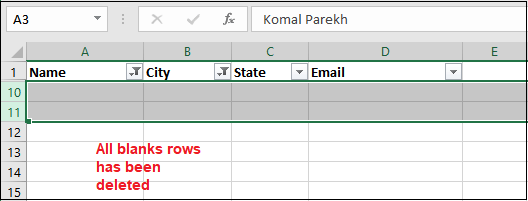
Step 10: Expand the row and see that – no blank row remained between the data rows.