

How to unhide columns in Excel?
The Excel users often hide the columns when they don’t want to show complete information stored in an Excel sheet. Hiding the columns is a solution rather than deleting them. A double line between two columns donates to the hidden columns in the header of the Excel worksheet.
When you hide a column, the data is not visible to the users but is not deleted. You can unhide the column and its data whenever you want the visible it again. This chapter will show the methods to unhide the columns in Excel.
How to let the user know that column is hidden
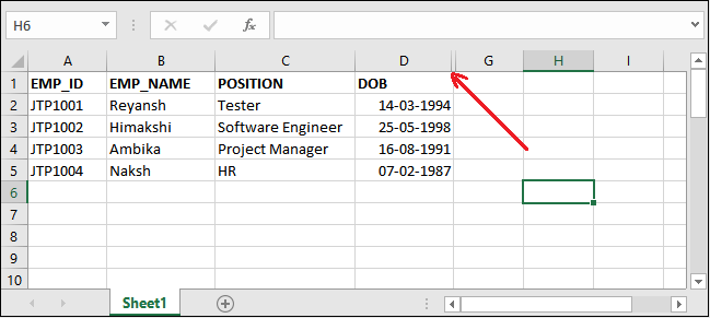
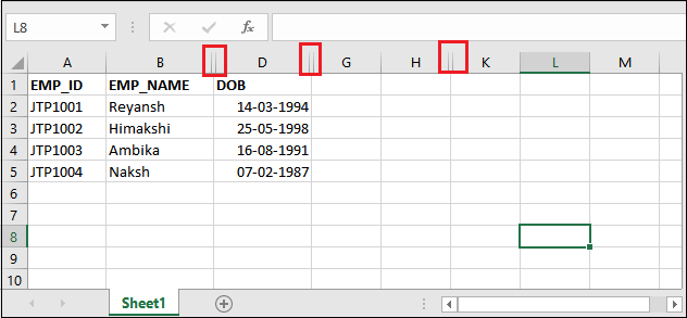
A double line between two columns donates to the hidden columns in the header of the Excel worksheet. See double lines in the below screenshot:
You can unhide the hidden column by increasing the size of the hidden column from the double line to the right.
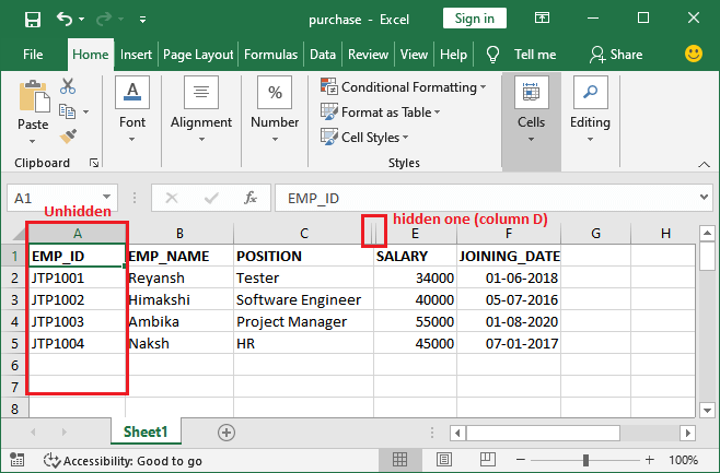
Additionally, there is one more way to know that the hidden columns. You can also get to know the total number of hidden columns by seeing the Excel column header.
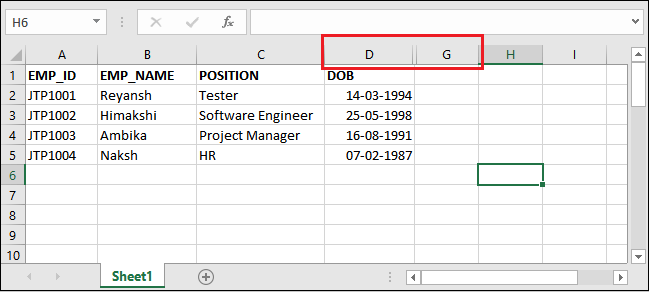
Look in the column header that we have column G just next to column D. It means that two columns (E and F) are hidden here.
Unhide the hidden columns
It is not so difficult to unhide the hidden columns. There are four different ways to unhide the columns using the standard Hidden option, Document Inspector, using a macro, or Go to special functionality. We will describe all these methods one-by-one in detail.
- Unhide selected hidden columns
- Unhide all hidden columns
- How to unhide first column (column A)
- Unhide the columns using VBA script
- Check the total number of hidden columns
Unhide the selected hidden columns
This is a standard method to unhide the selected hidden columns in an Excel worksheet. It requires only two simple steps. To unhide the selected column, we will use the Standard Hidden option.
We will explain these steps to unhide the hidden column in Excel to make the data visible to the users. Follow the steps below:
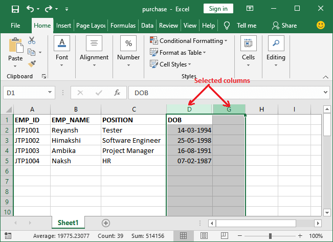
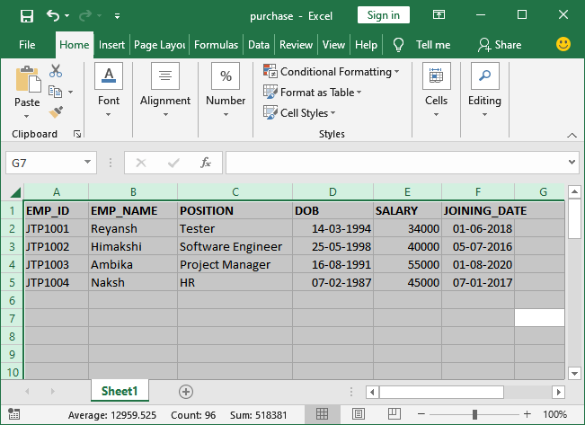
Step 1: Select the two columns (previous and next to the hidden one). For example, D and G here.
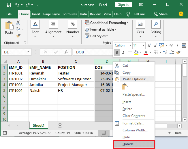
Step 2: Now, right-click on the selected columns and click on the Unhide option at the end of the list. That’s it.
Result
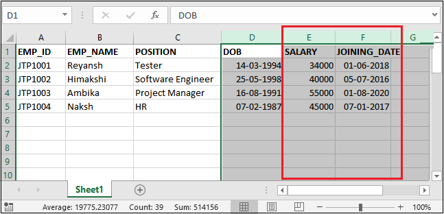
All the hidden columns between the selected ones will be unhidden, as you can see by yourself. See that column E (Salary) and F (Joining_Date) columns are visible now.
Unhide all hidden columns
It might be possible that two or more columns are hidden at different places, which can take time to find and unhide them. Thus, this time we will unhide all the hidden columns at once in an Excel worksheet. Whether there is one hidden column or more, this method will unhide all the hidden columns.
This method is also the same as the above some and two simple steps to be performed. We have a few steps to unhide all the hidden columns in Excel to make the data visible to the users. Follow the steps below:
Step 1: We have the following Excel dataset where more than two columns are hidden.
Step 2: In your Excel spreadsheet, click on the small triangle present at the start of the row and column in the upper left corner.
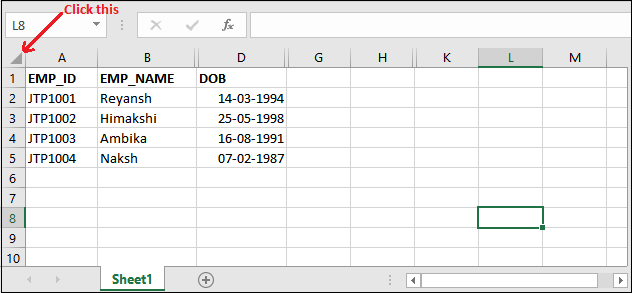
Tip: It will select the entire worksheet. However, you can also press the CTRL+A shortcut key for this.
Step 3: Right-click on the column header of the table, a context menu will open where click on the Unhide option.
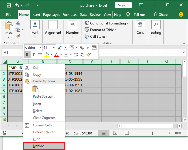
Note: If you clicked on selected cells rather than the column header, Unhide function would not work.
Result
As a result, all the hidden columns will unhide in the current Excel worksheet. Columns C, E, F, I, and J in one go.
Unhide the first column (A) of an Excel sheet
Often, the first column can also be hidden in an Excel worksheet and the user only want to unhide only that column, not all. Unhiding the columns seems easy, but when you need to display only the leftmost one, i.e., Column A, it requires a different method. There is no other column before the column A.
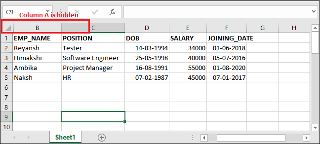
To unhide the first column (A) of an Excel sheet, we will use the Go To option. See how this option will use. We have the following Excel dataset where the first column A is hidden.
Now, follow the steps below:
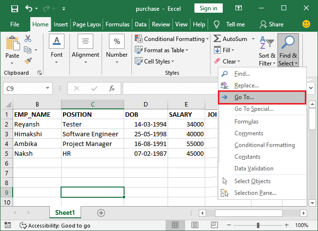
Step 1: On your Excel worksheet, navigate to Home > Find & Select > Go To to open the Go To dialogue box.
You can also use the F5 function key to open the Go To dialogue box directly.
Step 2: Under the Reference field, enter the column number, i.e., A1 and click the OK button.
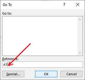
You cannot see, but cell A has been selected now.
Step 3: Now, in the same Home tab, go to the Cell group. In this cell group, click on the Format > Hide & Unhide > Unhide column.
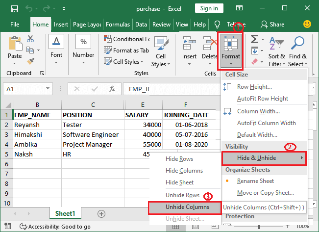
Step 4: Once you click on the Unhide column, column A will be unhidden. Note that – no other column will unhide, only column A (first column of the table) will unhide using this method.
See that column A is visible now and other hidden columns have not been unhide.
Increase the size of column of make it visible
Besides this method, you can also unhide a particular column (column A) by increasing the size of the column. Even you can apply this method for column A (leftmost column of the Excel worksheet). This method does not need any tricky steps to be performed. It just uses the mouse to drag the first column.
For this, take the mouse over the first column when the cursor looks like as showing in the below screenshot:
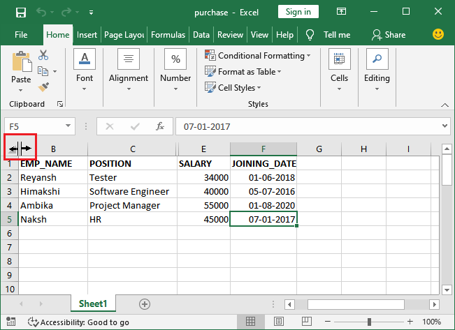
Double-tap to select it and then move this cursor to the right to increase the size of column A (first column).
It will look like something, as displaying below while dragging.
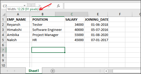
See that column A is visible now. Like this, you can unhide any other column in the Excel worksheet.

Unhide the columns using VBA script
Besides all the above methods, you can also use VBA to unhide the columns. VBA allows the users to write the code for this and execute that code to unhide the hidden columns.
It totally depends on the user if he/she wants to unhide the columns through coding. Use the following macro code (script) for it:
By executing this code in Excel VBA, all the hidden columns will be unhidden in your currently active Excel worksheet.
Similarly, if you also want to unhide the hidden rows, use the following script in VBA code:
Check the total number of hidden columns
In Excel, a user can find and count the total number of hidden columns in an Excel worksheet. Excel has an Inspect Document feature using which you can check the number of hidden columns. It will show detailed information about hidden columns and rows.
It is useful to inspect the number of hidden columns quickly. Here are a few steps to find the total hidden columns.
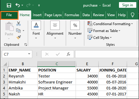
Step 1: Open the targeted worksheet and click on the File tab.
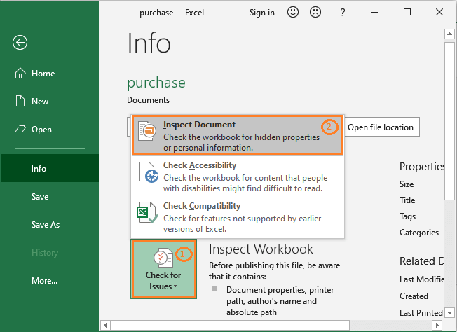
Step 2: In the left panel, firstly click on the Info option.

Step 3: Click on the Check for Issues dropdown option present just next to the Inspect Workbook and then click the Inspect Document.
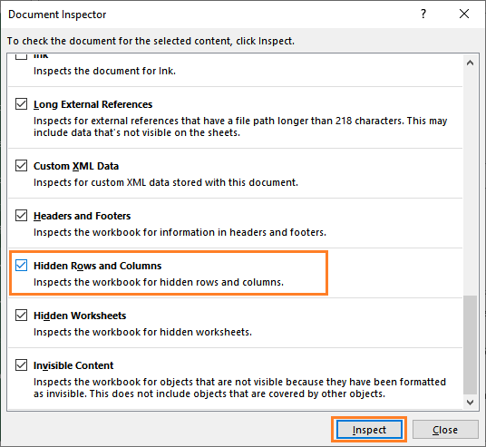
Step 4: In the document inspector panel, scroll down and verify that the Hidden rows and columns checkbox is marked. If not, mark it and then click the Inspect button below.
Step 5: Once again, scroll down and see the number of hidden columns/rows. It will show the number of hidden columns for the currently active Excel file.
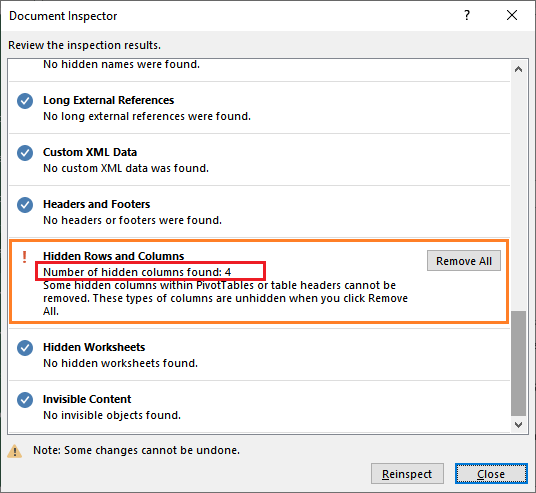
You can click the Remove All button to delete all hidden columns here.


