How to Use RIGHT Function in Excel

Right Function in Excel

The RIGHT Function is part of the Excel TEXT functions category. The RIGHT function will return a specified number of characters from the end of a given text string. It aids in the extraction of characters from the rightmost to the left side. The result depends on the number of characters specified in the formula. For example, “=RIGHT(“tutoraspire”,5)” gives “POINT” as a result.

The RIGHT function is helpful if we want to extract characters from the right side of a text string. Usually, it is used by combining it with other functions such as VALUE, COUNT, DAY, DATE, SUM, etc.

Syntax

The RIGHT function’s syntax is as follows:

Arguments

• Text(required):- The text string from which we need to extract characters.
• Num_chars: – Num_chars is optional. Specifies the number of characters we need RIGHT to extract.

1. num_chars must be greater than or equal to zero.
2. If num_chars is omitted, then it is assumed to be 1.
3. If num_chars is greater than the length of text, RIGHT returns.

Characteristics of the Num_Chars”

The following are the characteristics of the num_chars:

1. The default value of the “num_chars” is set at 1. It means the RIGHT function returns the last letter of the string if the value of “num_chars” is omitted.
2. The RIGHT function returns the #VALUE! Error if “num chars” is less than zero.
3. The RIGHT Function returns the complete text if “num chars” is larger than the length of the text.

Note

1. The RIGHT function might not be available in every language.
2. The RIGHT function is designed for languages that use the Single-Byte Character Set (SBCS). No matter what the default language setting is, RIGHT always considered each character as one, whether single-byte or double-byte.

How to Use RIGHT Function in Excel?

We mostly used the RIGHT function in combination with other Excel functions such as FIND, SEARCH, LEFT, LEN, etc.

The following are the uses of the RIGHT function:

• It helps format text.
• The RIGHT function removes the trailing slash in URLs.
• It extracts text which appears after a certain character.

Let us understand the use of the RIGHT function with the help of the following example:

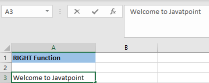
Example 1: In this example, there is a test string in cell A3, as we can see in the below screenshot. We need to extract the last word having 10 letters.

We will apply the RIGHT function in order to extract “string” in A3 column.

We will use the below formula:

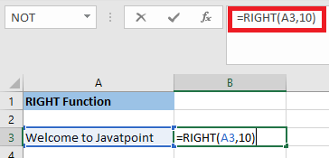
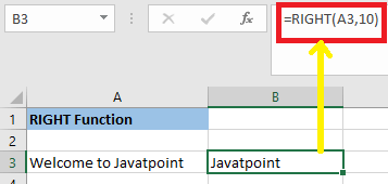
After applying the formula, the result would be:

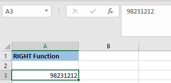
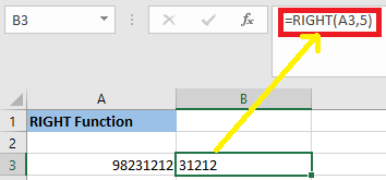
Example 2: In this example, we have an 8-digit number (98231212), and we have to extract the last 5 digits from this number.

In order to extract the last 5 digits, we have to apply the following formula:

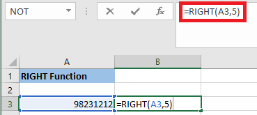
The RIGHT function returns 31212, as we can see in the below screenshot:

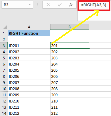
Example 3: In this example, we have a list of IDs such as “ID201,” “ID202”, “ID203”. “ID204,” etc., in column A.

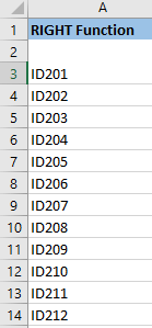
In this case, the last three digits of the ID are unique, and the text “ID” is redundant. As a result, we’d like to eliminate “ID” form the list of identifiers.

We will apply the below formula:

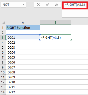
The RIGHT function returns 210 in cell B3. Using the same procedure, we will extract the last three digits of each ID.

Example 4: In this example, we have a dataset that contains invoice numbers. We want to extract the last 6 digits of each of the invoice numbers so, to do this, we have to use the RIGHT function.

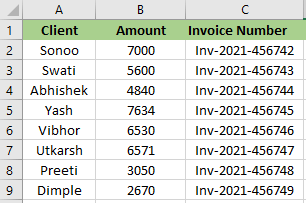
Using Excel’s RIGHT function, we can extract the last 6 digits of the above text.

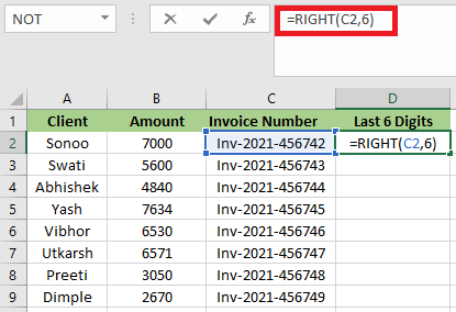
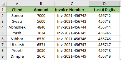
After applying the RIGHT function, the result will be:

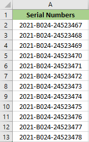
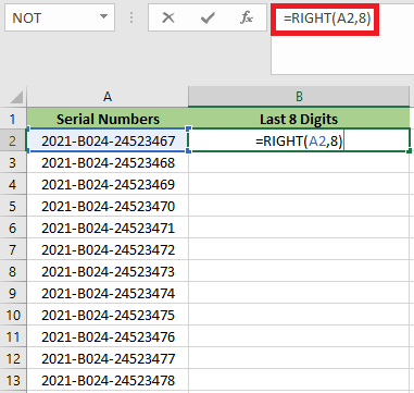
Example 5: Suppose we have serial numbers ranging from A2 to A13, and we want to extract 8 characters from the right.

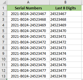
The RIGHT function returns the last 8 digits from the text’s right end.

After applying the formula, the result will be:

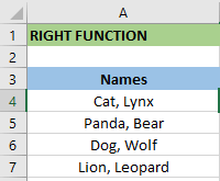
Example 6: In this example, we have the name of two animals in column A. Using comma and space, the names are separated, as shown in the below screenshot. We need to extract the last name.

In order to extract the last name, we have to use the following RIGHT formula.

• The “FIND(” “,A4)” finds the location of the space. It returns 5. Alternatively, we can use “,” for a stricter search.
• The “LEN(A4)” calculates the length of the string “Cat, Lynx.” It returns 9.
• The “LEN(A4)-FIND(” “,A4)” returns the position of the space from the right. It returns 4.
• The formula “RIGHT(A4,LEN(A4)-FIND(” “,A4))” returns 4 letters from the right of the text string in A4.

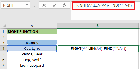
“Lynx” is the output of the RIGHT formula. The output for the remaining cells is also found in the same way.

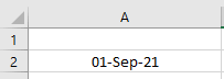
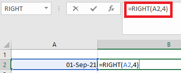
Example 7: Excel’s RIGHT function does not work with dates. Because the RIGHT function is a text function, it can also extract numbers, but it cannot extract dates. Let’s say cell A2 has a date “1-sept-2021”.

Now, we will try to extract the year with the help of the RIGHT formula.

The result would be 4440.

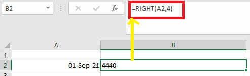
In excel. Ideology 4440 means 2021 if the format is in Dates. As a result, Excel’s RIGHT function will interpret it as a number rather than a date.

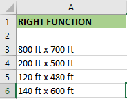
Example 8: In this example, we have 2-Dimensional data. The length is multiplied by the width, as we can see in the below screenshot. We need to extract the width from the given dimension.

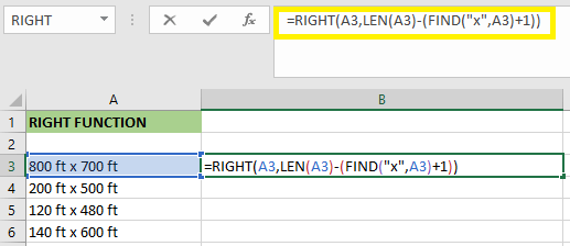
We will use the following RIGHT formula for the first dimension.

• The FIND(“x”,A3)” will return the position of “x” in the cell. It will return 8.
• The formula “FIND(“x”,A3)+11″ will return 9. We add one to omit the space because “x” is followed by a space.
• The “LEN(A3)” returns the string’s length.
• The number of characters that occur after “x”+1 is returned by “LEN(A4)-FIND(“x”,A3+1)”.
• The formula “RIGHT(A3,LEN(A3)-FIND(“X”,A3)+1))” returns all the character that occurs in one place after “x”.

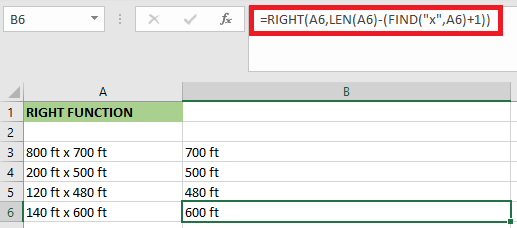
The RIGHT formula returns “700 ft” for the first dimension. We have to drag the fill handle to determine the results of the other cells.

Example 9: In this example, we have a list of email addresses. We need to extract the domain name from these email IDs.

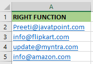
In order to extract the domain name from the first email address, we have to use the below RIGHT formula.

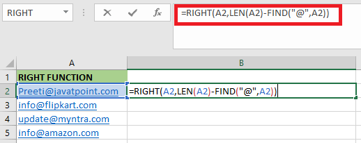
The length of the string A2 is given by “LEN(A2)”. It will return 21.

• The “FIND(“@”,A2)” will find the location of “@” in the string. It will return 7 for cell A2.
• The number of characters occurring to the right of “@” is given by “LEN(A2)-FIND(“@”,A2)).” It will return 14.
• The ” RIGHT(A2,LEN(A2)-FIND(“@”,A2))” returns the last 10 characters of cell B3.
  
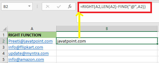
• The RIGHT formula returns “tutoraspire.com” in cell B2.
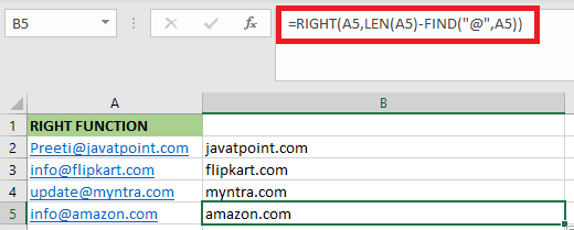
• In the same way, we will apply the formula to the remaining cells.
  

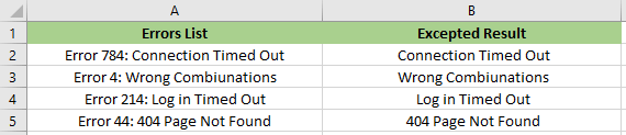
Example 10: In this example, there are some errors that we may encounter while using the web-based software are listed below. We have to extract substring after the last occurrence of the delimiter.

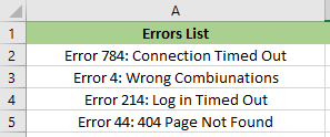
We can do this by using the combination of LEN, SEARCH and SUBSTITUTE along with the RIGHT function in Excel.

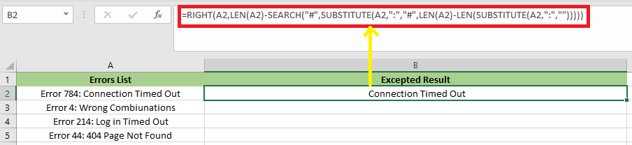
• First, we have to calculate the total length of the string with the help of the LEN function, which is LEN(A2).
• Then we have to calculate the length of the string with no delimiters, and we can calculate it with the help of the SUBSTITUTE function, which replaces all occurrences of a colon with nothing: LEN(SUBSTITUTE(A2,”:”,””))
• Next, we have to subtract the length of the original string with no delimiters, and we will use the following formula:

After applying the above formula, the result would be:

Things to Keep in Mind When Using the RIGHT Function:

The following are the things which we have to keep in mind when using RIGHT function:

• In Excel, the RIGHT function is used to extract characters from the right side of a text.
• The RIGHT function will not deliver exact results when it comes to date formatting.
• Number formatting is not a part of the string, and it will not be counted or extracted.
• In the case of complex data sets, we have to use other text function such as LEN, FIND, SEARCH and SUBSTITUTE.
• If the user doesn’t specify a value for the last argument, then it will take 1 by default.
• The number of characters in Num_chars must be more than or equal to zero. If the value is negative, then it will throw the error as #VALUE.