Linear Regression in Excel
 1. Click on Data (1), and then press on the Data Analysis (2).
2. Click on the regression.

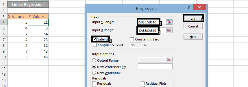
3. Select the cells for y-values (1), then the ones for x-values (2), and then check the labels (3). Finally, press ok (4).
4. Click on an empty cell (1), and then press insert (2). Press scatter chart (3), and choose a scatter chart (4).

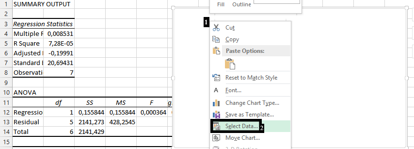
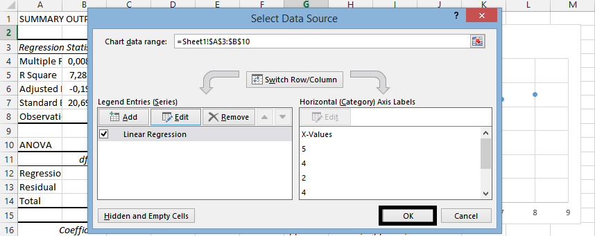
5. Right click on the chart (1), and choose Select Data (2).
6. Click Add.
7. Write the series name (1), choose the cells for X-values (2), and for Y-values (3). Press ok (4).

Note: The values are the data, which would be in another spreadsheet.
8. Click Ok.
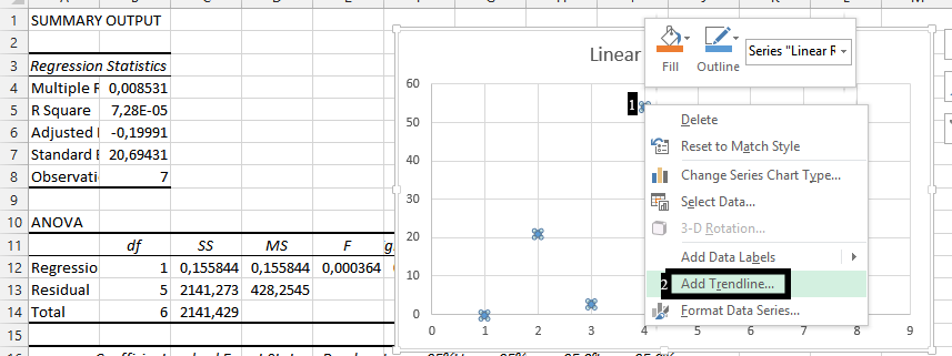
9. Right Click on any of the markers (1), and then select add trendline (2).
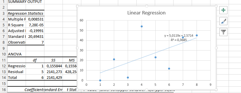
10. If you would prefer, check the Display Equation on Chart (1), and the R-square value on chart (2).

In conclusion, you should have done a linear regression that looks like this:
Template
Further reading:
Basic concepts
Getting started with Excel
Cell References


