The Only Match Function Tutorial You Need
MATCH function allows you to determine the position of the search item in the range of cells. Excel is mainly used as a database to store large amounts of data and frequently, you would have to search the Excel sheet for data. As it is not at all practical to search the data manually, Excel offers a few functions to search the sheet for a specific value like MATCH function.
The MATCH function returns the position of the searching value if successful and returns the #N/A error value if the function is unsuccessful.
How to use MATCH function?

Function syntax is as follows:
MATCH (lookup_value, range_lookup; [match_type])
- Lookup_value is an element we seek. This may be a number, text, logical value or cell reference that contains one of these types of data.
- Range_lookup a range of cells to be searched.
- Match_type is an optional argument (defaults to 1). It decides how to compare the values and looking for cells with the searched range. It may take the following values:
0 – the result is given as the first value in the field of equal sought,
1 – for sorted in ascending column gives the largest value less than or equal sought,
-1 – For sorted descending column gives the smallest value greater than or equal sought.
Match function example
Let us use the function in the following example:
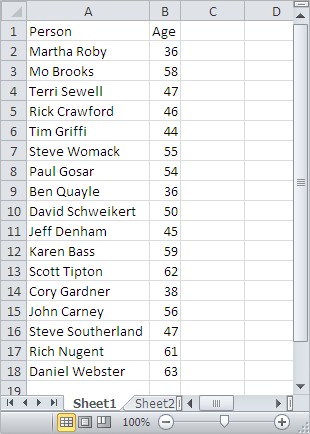
To find a person who is X years old, enter the following formula:
= MATCH (X, B2:B18, 0)
Looking for person at age 50, we obtain the result of 9 – and thus the ninth person on the list is 50 years old. Typing an analogous formula for a person who is 60 years old, we get an #N/A error. This means that the value was not found.

To use a comparison of 1, sort table columns ascending age. To find the oldest person whose age does not exceed X years, enter the formula:
=MATCH (X, B2:B18, 1)
Since the table is a person aged 50 years, the function returns its position. In the case of finding 60-year-old get the position of being 59 years old.
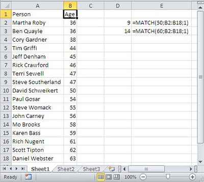
Let’s practice with these examples. Open Excel and save your file as match.xlsx. Enter details as in the following image.
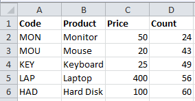
Example 1: Click the cell F1 and enter the formula
=MATCH(“MOU”,A2:A6,0).

Now the result is 2. The item MOU is in the second position in the array. We get the result as 2 because we started the array from A2 and the item is in the cell A3.
Example 2: Click the cell F2 and enter the formula
=MATCH(“MOU”,A1:A6,0).

Now the result is 3. The item MOU is in the third position in the array as we started the array from A1 this time.
Example 3: Click the cell F3 and enter the formula
=MATCH(“Har*”,B2:B6, 0).
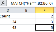
Now the result is 5. Here we use an asterisk to match any sequence of characters.
Example 4: Click the cell F4 and enter the formula
=MATCH(“Har?”,B2:B6, 0).Now your screen will look like this:
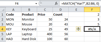
Here, you get the result as #N/A. The question mark matches a single character and there is no item with a single character after Har and hence it returns #N/A.
Example 5: Click the cell F5 and enter the formula
=MATCH(“LA?”,A2:A6, 0).
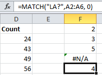
Now the result is 4. Here we use a question mark to match a single character.
Example 6: Click the cell F6 and enter the formula
=MATCH(48,D2:D6, 1).
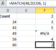
Now the result is 2. Here as the value of type parameter is 1, the position of the largest value that is less than or equal to 48 is returned.
Example 7: Click the cell F7 and enter the formula
=MATCH(62,D2:D6).
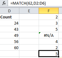
Now the result is 5. Here as the value of type parameter is omitted, it has the default value 1. Hence, the position of the largest value that is less than or equal to 62 is returned.
Example 8: Enter details in the A column as in the following image.

Click the cell F8 and enter the formula
=MATCH(68,A9:A15,-1).
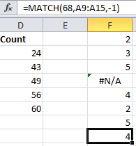
Now the result is 4. Here as the value of type parameter is -1, the position of the smallest value that is greater than 68 is returned.
Example 9: Click the cell F9 and enter the formula
=MATCH(43,A9:A15,-1).
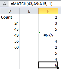
Now the result is 6. Here as the value of type parameter is -1, the position of the smallest value that is greater than 43 is returned.
Example 10: Click the cell F10 and enter the formula
=MATCH(87,A9:A15,0).
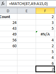
Now the result is 2. Here as 87 is repeated twice in the array, it returns the position of the first instance of 87.
Match function business examples
Let’s move on with more business examples of MATCH function usage.
Example 11: Simple Match Formula
We are using a match formula to find out if the price has been set for a product.

Example 12: Where is a Product?
The business’ products have been layout in a Microsoft Excel. We are now trying to find out where a product is in the list. Thanks to Match function in Excel, it is very easy to find it.

Example 13: IF and MATCH
The product has been listed. But, we are trying to find out the price of the product. But, we’d know the price of a product, and we’d want to answer if the price is right. This is why we find IF and MATCH formulas useful.

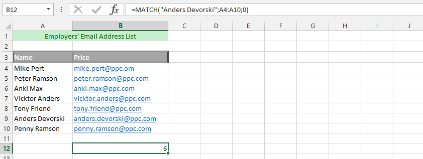
Example 14: Finding Employee with MATCH
The employees are quite many. But, the executive do not know all of them, and would like to find what row the employee has a name, and we could not find out the email. There are other functions that could be used for finding it, but we prefer using the match to find out the row. This was meant to find out what row to go to, in order to get the email of that employee.
Example 15: Double Match Formula
We’d know the name of the product, but we don’t know if the price was correct or if they are on the same row. This made us worried about acknowledgement of the inputted information, which is why we find MATCH function in Excel to be very useful for verifying that the data is both completed and in the same row. We are now going to use double MATCH formula to find the answer that we are looking for.
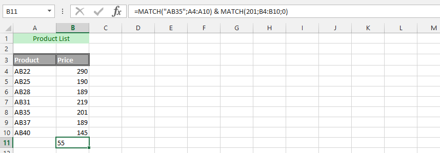
Example 16: Did we Send Right Details and Information?
We are sending a product to a customers. The price has been set, but due to a specific deal we made with the client, we would like to make sure that the price was correct. We have determined that the client would only get to pay a specific amount of money, which is why we will use the IF and double match formula.
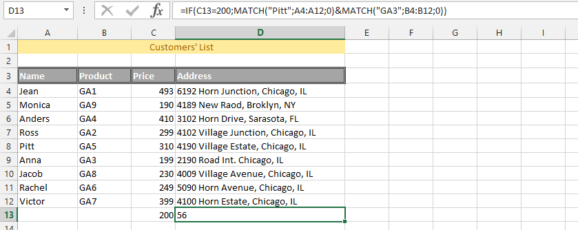
Example 17: Is Everything in The Same Row?
It is easy to list all the products that are being sold. But, the company has just fired one of its workers for inadequacy in their performance, and one of them was that they frequently miss one critical details that will end up costing the company money. The employee would not miss something small, but he would put 100 dollars beside a product that cost 1500. This is why we are going to use triple MATCH formulas to ensure that the expensive products have right layout. These would allow me to ensure that everything is in order.
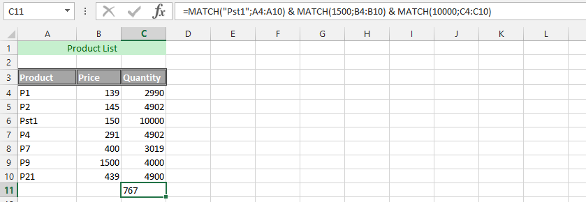
Example 18: Complete Text
The whole data has been layout as text, and we are looking for a product. We are using the same data as previous one.
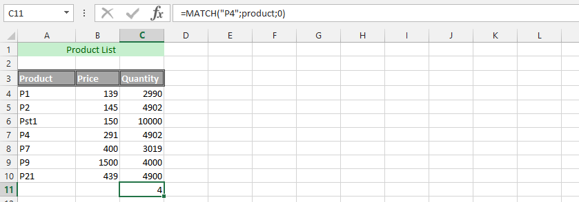
Example 19: Is Our Product in Another Spreadsheet?
We have now gone from having our data in one sheet, and would like to verify that the same data in one is matching the other.

Example 20: Information from another Document
The situation is that we have our data ready, and now we need to find the solid correspondent between both data, so we could determine if our data has been solid. We’d have the previous year in another document, and this year is in the current one, which is why we need to verify that the data is coherent. It is about acknowledging that the total is there too, so we could find it.

Template
Further reading:
Basic concepts
Getting started with Excel
Cell References


