Modifying A Calculated Field In A Pivot Table
You need this to make proper calculation which you need at the moment.
1. Open sheet with your pivot table and click any cell in the pivot table to get it activated.

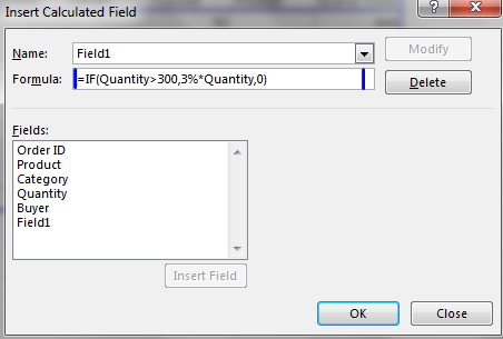
2. Go to Analyze tab. Select Fields, Items and Sets button and click Calculated Field.
3. A dialog box will appear. Enter the formula as per your requirements. (Marked with blue in the following screenshot):

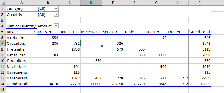
4. Click ok. Excel will display the pivot table with an additional column (sum of discount in this case).

5. Click anywhere in the pivot table. PivotTable Fields appears on the right. Under sum of values, go to sum of quantity and click remove field.
Final result will be like this:

As you see you have Sum of Discount instead of Sum of Quantity. Now you know how to modify calculated field in Pivot Tables. Use this to make your customized calculations.
Template
Further reading:
Basic concepts
Getting started with Excel
Cell References


