

Offset function in Excel
Offset() is an Excel function that is used to get the reference of a range and return back to the user. It is a bit tricky function and not so easy to understand and use. Once you learn and get it, you can use it on your Excel worksheet easily.
Note: The resultant value can be a single cell or range of multiple adjacent cells.
This chapter will brief you on the offset function functionality with its syntax and examples. You can find this LOOKUP function (user interface) under the Lookup & Reference list inside the Formula tab in Excel. Follow our complete tutorial.
Use of offset()
Using the offset() function, you can directly move to a cell in any direction (left, right, up, down, as well as diagonally). For example,
A rook can move only straight in left, right, up, and down, not in diagonal on a chessboard,. Similarly, using other functions of Excel, a user can straight go to a cell. The offset() function enables the users to move diagonally.
Syntax
Here is the syntax of the offset() function. It accepts five arguments in it.
Provide a starting point in reference parameter and number of rows and columns to move left, right, and up, down. While height and width are optional.
Parameter list
The OFFSET() function have five parameters in which first three are mandatory, and others are optional parameter –
Required arguments
reference (mandatory) – It is the starting point, which is used as a range or call reference. E.g., A2, B5, etc. It is the base cell.
rows (mandatory) – The number of rows above or below from the starting reference value. It can be a positive or negative number.
column (mandatory) – The number of columns left or right to the starting reference value. This parameter can accept positive or negative values.
Optional arguments
[height] (optional) – The height parameter is passed to get the number of rows to be returned. This parameter accepts only a numeric value, and it must be a positive number.
Usually, this parameter is used to get the multiple values to be returned.
For example., If the height is 1, only one row data will return. But if the height parameter value is 2, then the targeted cell and its below cell data (multiple values) will return.
[width] (optional) – The width parameter is passed to get the sum of the number of columns to be returned. Like the height parameter, it also accepts only a numeric value, and it must be a positive number.
E.g., If the value is 2, sum of the selected cell (selected by the first three mandatory parameters) + and cell in the next column will return.
Note: You can use the OFFSET() function inside another Excel function to handle the multiple values returned by it on using the height and width parameter.
Now, we will illustrate the theory in practical and with the help of example, you will get it better.
Return Value
The OFFSET() function returns a reference to the range. This reference can be a single cell or multiple cells.
OFFSET Warning
The OFFSET() function is a volatile function. If it is applied on too many cells in an Excel workbook, it can slow down the processing of that workbook. Thus, you can use other Excel functions instead of it to keep the processing faster.
Excel offers a non-volatile function to return a reference, like INDEX(). It does not slow down the process of the workbook.
OFFSET Example
Before start learning the OFFSET function directly on an Excel worksheet, try to understand it with the help of syntax examples. See some OFFSET syntax as the examples below:
| Formula | Description |
|---|---|
| =OFFSET(A2,4,3) |
The resultant cell value will be D6. |
| =SUM(OFFSET(A2,2,4, 1,1)) |
The resultant cell value will be E4 only. Nothing will be summed up because the selected cell is only E4. |
| =AVERAGE(OFFSET(A2,2,4, 2,1)) | Like the above example,
Firstly, the cell E4 will be selected using the first three parameters. Then, using the optional parameter, one more cell (E5) in the next row will select. |
Need of Offset() function
The offset() function is very helpful in the dynamic calculation. Let’s understand using an example that why this function is needed. We have a problem that is resolved by offset().
Problem
We have a set of data of 7 days in which we want to calculate the average of the last 5 days. This can be easily done using the Average formula (=AVERAGE(B3:B7)) of Excel.
But the problem is – we have added one more row (B8) in the end and again calculated the average of the last 5 days. In this scenario, we have to change the range of the targeted column, and the average formula will be (=AVERAGE(B4:B8)). The resultant value will also be changed now.
Solution
This problem can be resolved using the offset() function. It enables the users to get the reference of the cell and then calculate the SUM, AVERAGE, or other operation with it by selecting multiple values using its optional parameters. For example,
=AVERAGE(OFFSET(A2,5,3,2,1))
How OFFSET() function is used?
With the help of different examples, you will now see how the OFFSET() function is used. For the example of the OFFSET() function, we have the following set of data of one month.
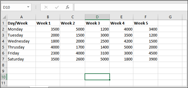
We have this worksheet containing the weekly report of each day in one month. We will now apply the OFFSET() formula on this worksheet.
Without height and width parameter
Example 1
Step 1: Select a cell to keep the result returned by the OFFSET() function and apply the following OFFSET() formula by writing it in the formula bar.
=OFFSET(A2,4,3)
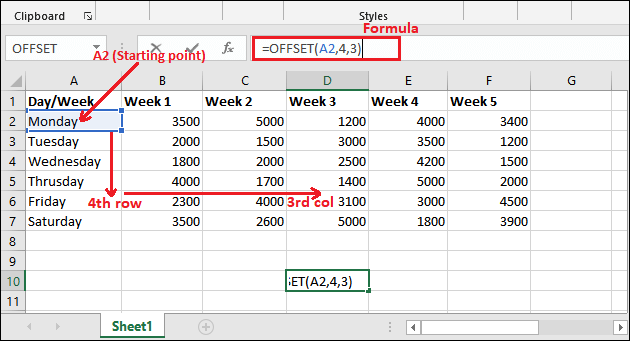
Step 2: After writing the OFFSET() formula inside the formula bar, click the Enter key to get the resultant value.
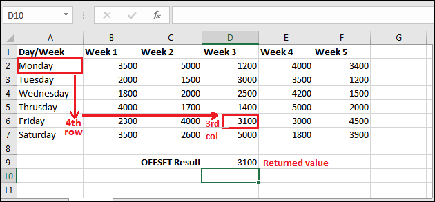
See that the 3100 has been returned on executing the OFFSET() function. In this example, we have only used the first three mandatory parameters.
Example 2
See one more example of offset() function without having height and width parameters. We will use the same data table for this example and only arguments are changed.
Step 1: Select a cell to keep the result returned by the OFFSET() function and apply the following OFFSET() formula by writing it in the formula bar.
Offset Formula
=OFFSET(A1,2,3)
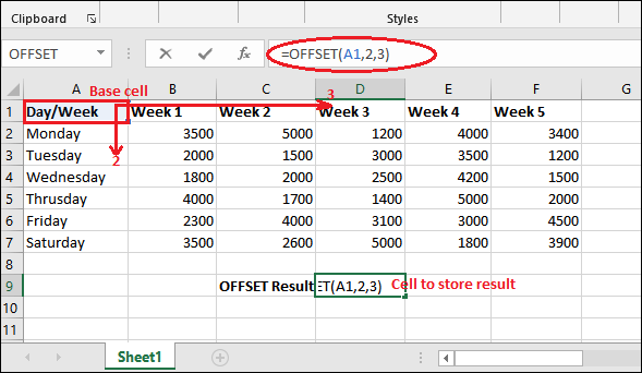
Step 2: After writing the OFFSET() formula inside the formula bar, click the Enter key to get the resultant value.
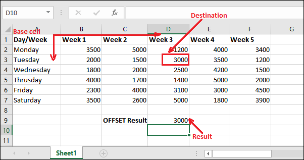
See that the offset() function has been returned 3000 on executing the OFFSET() function.
Using height and width parameter
In this example, we will use the height and width (optional) parameters in the offset() function. See how differently its outcome receives.
The offset() function usually returns multiple values, which is hold by using another function. This means you have to pass the offset() inside another function to hold the values returned by it.
Example 1
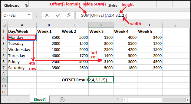
In this example, we will use this OFFSET() function inside the SUM() function to get the sum of values (reference cell) return by the offset() function. Here, we will use it for cell selection from multiple rows by entering the height value to 2.
Steps to calculate sum with offset
See the few simple steps for it below:
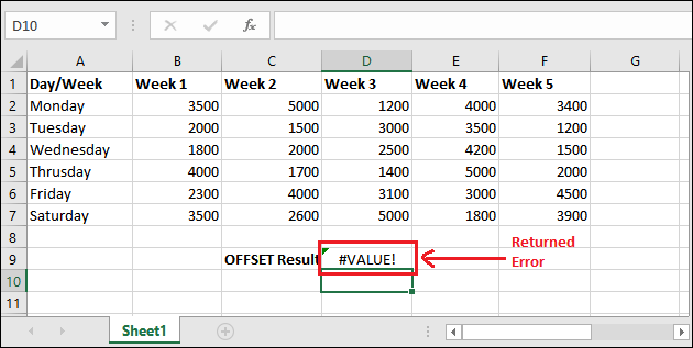
Step 1: Like the above example, select a cell to keep the result returned by the OFFSET() function and apply the following OFFSET() formula with height and width parameter by writing it in the formula bar.
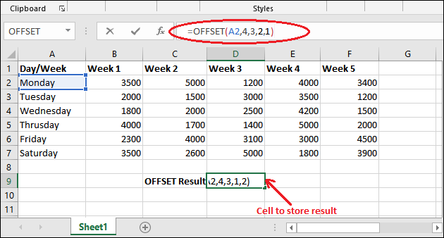
Step 2: Now, press the Enter key. It will generate a #VALUE! error as more than one value has returned.
Step 3: To handle this error, we will put this formula inside another function. We will use the SUM() function that will return the sum of the cells choose by the offset() function.

Step 4: After writing the OFFSET() formula inside the formula bar, click the Enter key to get the resultant value.
See that it has returned the sum of the cells (D6, D7) whose reference return by the offset().
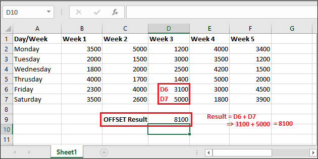
The sum has returned, i.e., 8100. You have now got this how the offset function works with optional parameter.
Example 2
See one more example of the offset() function with the optional parameters (height and width). In this example, we will use the offset() function inside the AVERAGE() to get the average of values (reference cell) return by the offset() function.
This time, we will use it for cell selection from multiple columns by entering the width value to 2.
Steps to calculate sum with offset
See the few simple steps for it below:
Step 1: Select a cell to keep the result returned by the OFFSET() function with SUM() and apply the following OFFSET() formula with height and width parameter by writing it in the formula bar.
Step 2: The offset() will return the reference of D6 and E6 cell as the width is 2. So, two cells reference will return whose sum will calculate and return.
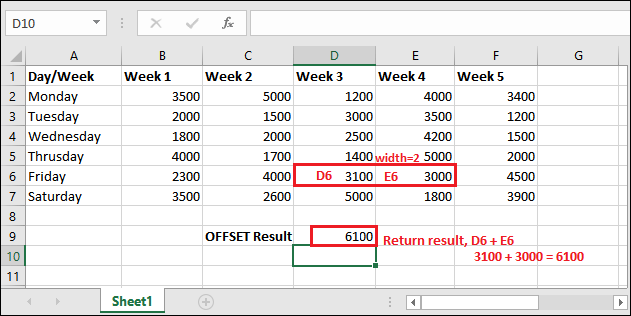
By using the above offset() formula with SUM() function, calculated result 6100 has returned.
Example 3: Sum all cells of a column
There are 5 columns containing 5 weeks of data in this Excel table, where each column contains 6 days of data. Illustrate an example to sum all cells of a column using the offset() function.
Step 1: Use the following offset() formula inside the SUM() to get all cells summed up of a column.
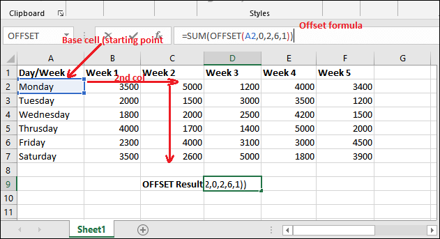
It will go for the same row and the second column from the starting point, then calculate the sum of six cells of that column.
Step 2: Press the Enter key and the sum of six cells of column C (reference return by offset()) will return to the selected cell. Look into the output below:
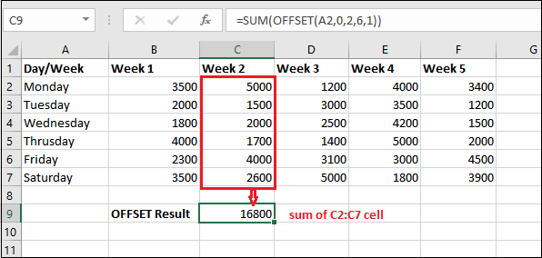
Here, the sum is calculated through the offset() function.
The offset() function is probably the most confusing function in Excel.
Example 3: Sum the cells of a row
In this Excel table, you can see that there are 7 rows containing 6 different days data, where each column contains one week of data. With the help of a simple example, we will illustrate to sum the all cells (that contains some data) of a row using the offset() function.
Step 1: Use the following offset() formula inside the SUM() to get all cells to be summed up in a row.
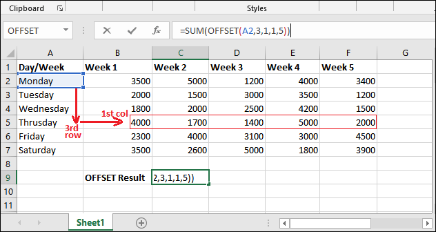
It will go for the fifth row and the first column from the starting point, then calculate the sum of five cells with respect to the fifth row.
Step 2: Press the Enter key and the sum of five cells with respect to the 5th row (reference return by offset()) will return to the selected cell. Look into the output below:
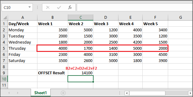
Here, the sum is calculated through the offset() function.


