Range in Excel

Whenever we see the word range in excel, we refer to it as a cell or a collection of cells in an excel spreadsheet. It can also be used to refer to the adjacent cells or non-adjacent cells in the dataset. In excel, each range has its defined set of coordinates or positions, unlike A4:A7, B5: F9C, etc.

You can perform many operations with ranges in your Excel worksheet, unlike copying the dataset, moving data from one position to another, formatting cells, and even you can name your range. In this tutorial, we will briefly cover all the topics about ranges.

Select a Range

While working with excel, you may want to select a multi cell range so you can easily make a command for all the cells at once. For example, let’s suppose you can highlight the headers in the cell range A2:E2. You select the range and change the background colour of the cells.

Following are the steps to select a range in Excel:

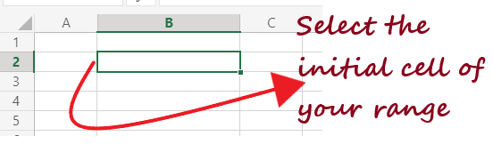
A. Select contiguous range of cells

1. Select the cell from where you want to start selecting your range. In our case, we have selected the B2 cell.
   
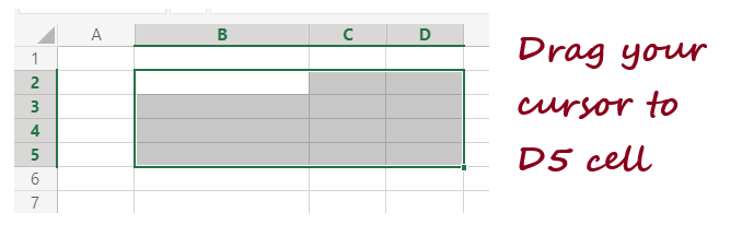
2. Drag your cursor to the last cell of your range. As you can see, we have dragged our pointer to the D5 cell.
   
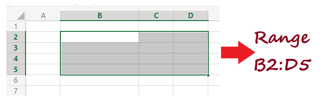
3. Hence the range B2: D5 got selected.
   

Similarly, you can select any range of cells in your Excel worksheet.

B. Select non-contiguous range of cells

1. Select the cell from where you want to start selecting your range. In our case, we have selected the B2 cell.
   
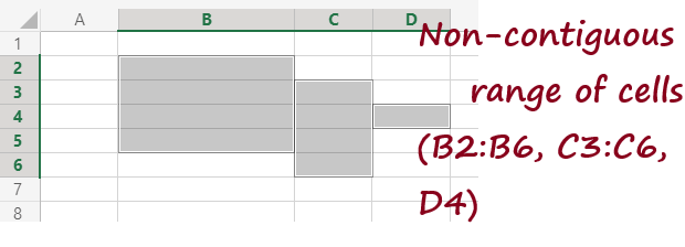
2. Hold the ‘CTRL’ key on your select and the various non-adjacent cells. We have selected B2:B6, C3:C6, D4 range of cells.
   

Types of Ranges

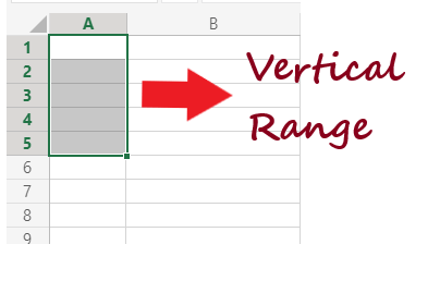
1. Vertical Range
   Vertical range refers to the selection of the cells within a column. For example, in the below image, the vertical range is A1:A5. However, if you select the entire column, the vertical range would be A: A.
   
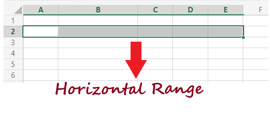
2. Horizontal Range
   Horizontal Range refers to the selection of cells within a row. For example, in the below image, the horizontal range is A2:E2. However, if you select the entire row, the vertical range would be 2:2.
   
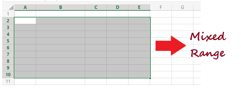
3. Mixed Range
   Mixed Range refers to the collection of cells formed by combining adjacent rows and columns. For instance, in the below example, the mixed Range is A2: E10.
   
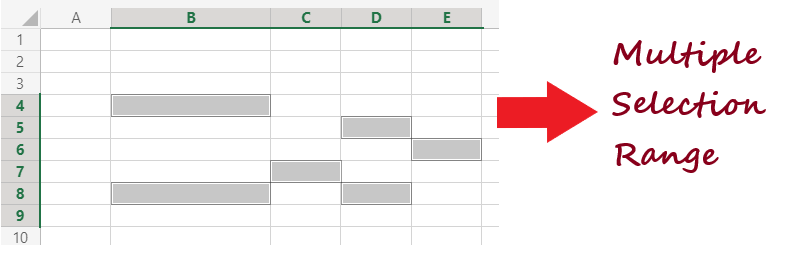
4. Multiple Selection Range
   To define a range, it’s not necessary to select only the adjacent cells. Therefore with Multiple Selection Range, a collection of non-adjacent cells are selected. For instance, in the below example the Multiple Selection range is B4, B8, C7, D5, D8, E6.
   

Move a Range

By default, if you move a range of cells in excel, it will move the data from one location to another along with its formatting such as font, text or number format, cell borders, font colour, etc.

Follow the given below steps to move a range of cells in Excel:

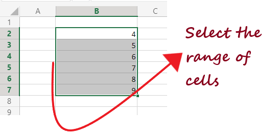
1. Select the range of cells you want to move from one location to another in your excel spreadsheet.
   
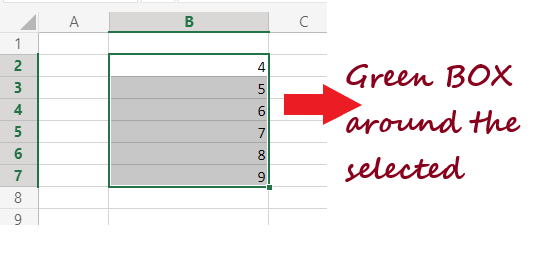
2. As soon as you select the cells, you will notice the entire range of selected cells become active with a green box around it.
   
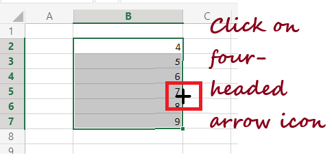
3. Move your cursor to the green border, and you will see that the cursor changes to a four-headed arrow icon.
   
4. Using the arrow moves the cell to another location within the same Excel worksheet. Unlike here, we can move it to column E.
   

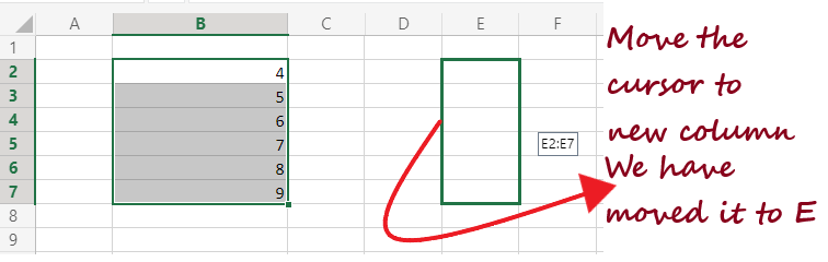
Note: After moving the cells, all the data and formatting will be automatically removed from the original range (C1:C6).

Copy/Paste a Range

By default, if you copy a range of cells in excel, it will copy the data from one location along with its formatting such as font, text or number format, cell borders, font colour, etc. and paste it to its new location.

Follow the given below steps to copy & paste a range of cells in Excel:

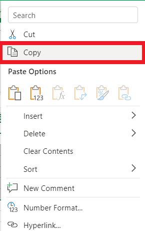
1. Select the range of cells that you wish to copy.
   
2. Put your cursor on top of your selected cell and right-click on it. The following window will be displayed. Click on the Copy option. Or you can directly press the shortcut key, i.e., CTRL + c.
   
3. Select the cell from where you want to start pasting the copied cell. Either right-click on the cell and select the paste option or press the ‘CTRL + V’ option directly.
   

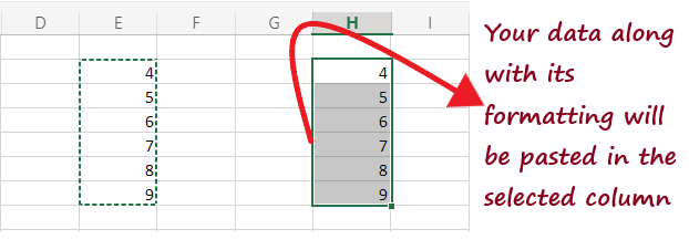
That’s it, your data (along with its formatting) will be pasted to the new location of your excel spreadsheet.

Note: You will notice that the selected range of cells (B1:C6) still has a dotted border. It means the excel range is still copied in your clipboard, and you can again paste it anywhere within your excel worksheet. Therefore we need to remove the data from our clipboard. To clear the clipboard content, press the Escape key from the keyboard. And as soon as you do that, the dotted border about the range will longer be seen.

Named Range in Excel

A named range is an amazing excel feature used to define the name for a collection of cells or ranges in a worksheet. Named range works as an added advantage as it helps to calculate functions and formulas quickly.

To add a named range in your Excel worksheet, follow the below steps:

1. Select the range of cells for which you want to define the name.

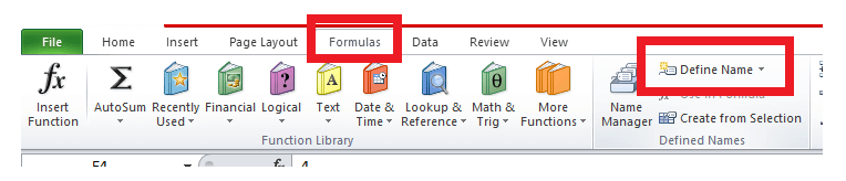
2. Go to the ribbon toolbar located at the top of your Excel window. Click on the Formulas tab -> Defined Names group -> Define Name option.

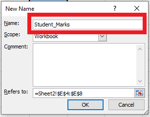
3. The New Name window will open (as shown below). In the descriptive name textbox, enter any suitable name for the range. In our case, we have entered Student_Marks as the name for the selected range.

Note: The name textbox can hold only up to 255 characters.

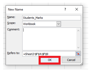
4. After specifying the name, it’s time to specify the range of cells from which you want to apply the name; therefore, in the “Refers to” box, select the range from your Excel worksheet.

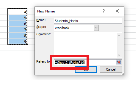
5. Once done, click on the OK button.

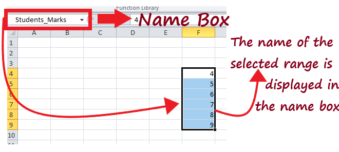
6. The window will be closed, and when you return to the spreadsheet, you will notice the name Students_Marks is highlighted in the Name box for the selected range of cells (as shown in the image below).

Note: If you have named any range, you will see the range name in the Name box whenever you select that column.

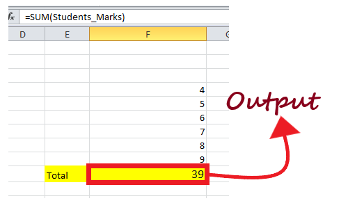
7. Now that we have defined the range’s name, we can directly use the name Student_Marks in formulas to refer to the named range of cells. For example, type the below formula in your excel worksheet.

Formula used:

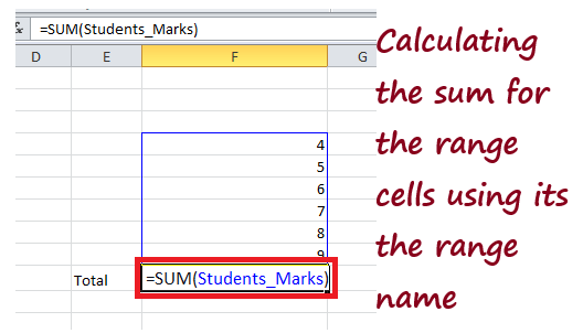
8. The SUM formula will quickly calculate the sum of all numbers present in a defined range and will give you the following result.