Regression analysis in Excel

The regression analysis is a part of statistical modeling that is used to estimate the relationship between the two or more variables. In MS Excel, you can perform several statistical analyses, including regression analysis. This one is a good option because almost every computer user can access Excel.

Excel provides the inbuilt method to calculate the regression. In MS Excel, regression feature is available at the end inside the Data tab. You have to add this Data Analysis ToolPak exclusively to your Excel from Add-ins.

Note: Excel users do not need to install the Data Analysis ToolPak from the internet. It is available in the Add-ins.

Before going in deep, you must know – what is regression analysis? Types of variables in it and many more basics things. We will explain all these terms in this chapter. So, go through the chapter till the end.

What is regression analysis?

Regression analysis is an analysis that shows a relationship between dependent and independent variables and produces an equation. This equation consists of a coefficient that represents the relationship of dependent and independent variables.

Simple Linear Regression

In simple linear regression, the value of one variable is used to describe the value of another variable. The variable that is being described is called dependent variable, while the variable, which is used to describe or predict the value of dependent variable is called independent variable.

Note: Independent and dependent variable are the two most essential terms of regression analysis.

Types of variables in regression

Regression analysis have two variables:

1. Dependent variable (predictor variable)
2. Independent variable (explanatory variable)

Dependent variable is the factor that we try to understand and predict. The value of dependent varies according the independent variable. In contrast, independent variables are those factors that affect the dependent variable and helps to predict the value for dependent variables.

Real Scenario

Let’s take a scenario to understand the variables of regression analysis –

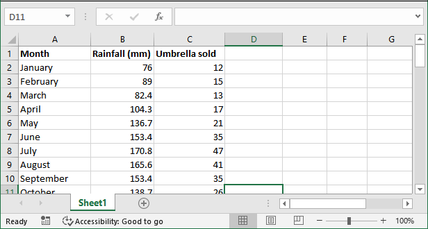
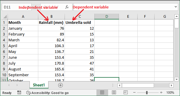
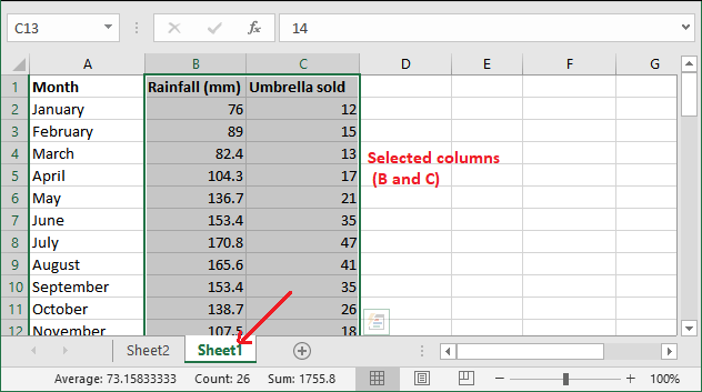
For example, we have sells data of 12 months stored in an Excel worksheet. This data is for the sell of umbrellas from January to December. Each month sell is different according to rainfall. Umbrellas are most sold in month July and less sold in January.

This Excel worksheet will contain three columns: Months (Jan to Dec), Rainfall percentage, and sold umbrella quantity (total number of umbrellas sold in each month).

Here,

Dependent variable: Umbrella

Independent variable: Rainfall percent

So, the umbrella is a dependent variable whose sell depends on the rainfall percentage of each month, which is an independent variable. Sell of umbrellas increase and decreases when rainfall is high or low. Hope you have understood the dependent and independent variable in regression analysis.

Verify Data Analysis ToolPak is installed

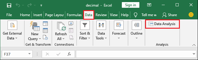
Now, before proceeding forward, verify that the Data Analysis ToolPak is enabled and available inside Data tab. Go to the Data tab and check for the Data Analysis ToolPak inside the ribbon at last. See in screenshot below:

If it is not enabled, add it to your Excel for performing regression analysis.

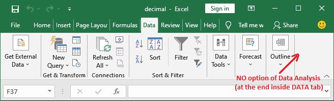
If the Data Analysis option is not available as shown in above screenshot, add it to your Excel by following below steps explained below in detail.

Enable data analysis ToolPak

Follow the steps to enable the data analysis ToolPak inside the Data tab.

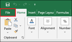
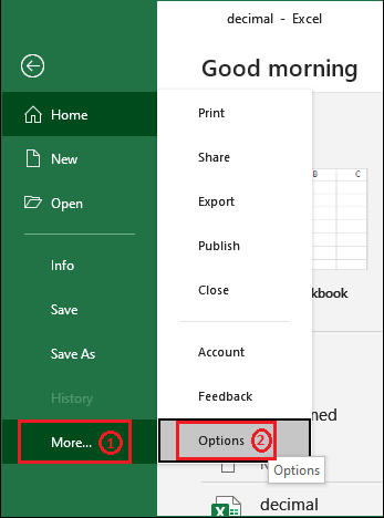
Step 1: In your current active Excel worksheet, go to the File in Excel menu bar.

Step 2: Inside the More? in left sidebar, you will see an Options option. Click on it that will open a panel containing various settings.

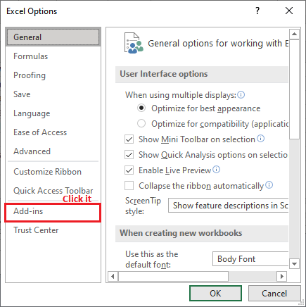
Step 3: From the Excel options panel, click on the Add-ins in the left sidebar.

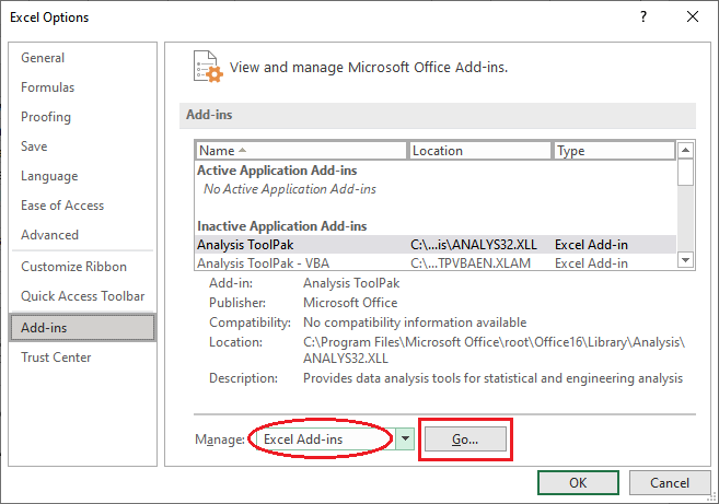
Step 4: Here, verify that the “Excel Add-ins” is selected inside the Manage dropdown list. If yes, click Go next to the dropdown button.

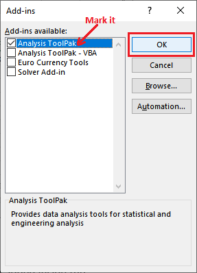
Step 5: In the Excel Add-ins dialog box, mark the Analysis ToolPak and click OK.

Step 6: Close all the extra tabs opened and see that the Data Analysis ToolPak has been added inside the Data tab.

Now, your Excel is ready to do regression analysis on data. Thus, we will now perform regression analysis on the scenario defined above.

Apply regression analysis

Now, you will see how regression analysis is performed on the Excel data step by step. We have this data here.

Step 1: Inside the Data tab, click on the Data Analysis option added it Excel in earlier steps.

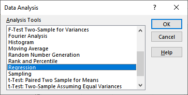
Step 2: Scroll down and Select the Regression from the list and click OK in this panel.

Step 3: Now, configure the following settings in the regression dialogue box.

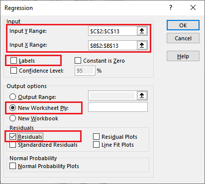
• In Input Y range, provide the cell reference of dependent variables. In our dataset, umbrella is the dependent variable that resides in column C. So, the cell reference will be C2:C13.
• In Input X range, provide the cell reference of independent variables. For example, in our dataset, rainfall is the independent variable resides in column B. Hence, the cell reference will be B2:B13.
• Mark the Labels checkbox if you have included header cell reference in X, Y ranges.
• Carefully choose an output option from here. We have chosen New workbook Ply.
• In the end, mark the residuals checkbox that will provide you the difference between actual and predicted values.

Step 4: Enter all these required details carefully and click OK.

It will generate a summary in Sheet2 for the analysis after setting up the following things.

Step 5: See the output created by Excel regression analysis and observe it.

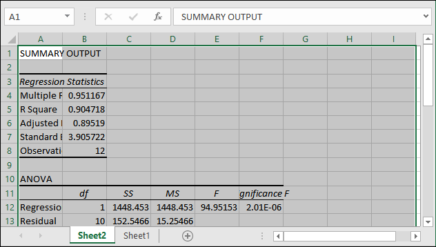
This summary output will contain REGRESSION STATISTICS, ANOVA, and RESIDUAL OUTPUT, most importantly. All these details in the same page.

Interpret the regression analysis result

We have performed regression analysis and you have noticed that the execution of regression is very easy. You have to do nothing difficult with it because all the calculations take place automatically. The complete output is auto-generated along with the statement as well.

Calculation is easy, but the interpretation is not so easy to understand. So, this time is to interpret its result. You have seen that the output is containing four major parts: regression statistics, ANOVA, and residual output. Let’s analyze them:

Regression Statistics

Regression statistics tell you how the linear regression equations fit in our data.

Let’s understand the terms used in the regression statistics table.

• Multiple R is the correlation coefficient that helps to measure the strength of a linear relationship between two variables. The higher value of Multiple R means the stronger relationship between variables.
  1: Strong positive relationship
  -1: Strong negative relationship
  0: No relationship at all.
• R Square is the coefficient of determination, which currently has its value 0.9047. It represents the goodness of fit. Round off the first to digits which will be 90% that is fair enough to fit in our regression model. It means 90% of dependent variables are explained by independent variables.
  Generally, high values are better for R Square.
• Adjusted R Square is advanced of R square, which is adjusted for the number of independent variables. It is used for multiple analyses.
• Standard Error is also a goodness-of-fit measure. The regression equation will be more certain for the smaller number.
• Observation is the total number of observations in your model.

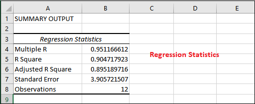
ANOVA

The next part of regression analysis is ANOVA, an analysis of variance. Then coefficient section with ANOVA.

• Df refers to the degree of freedom. It associates with the source of variance.
• SS refers to the sum of squares.
• MS is mean square.
• F is f statistics that test the overall significance of the model.
• Last one is Significance F that is the P-value of F.

The most essential component after the ANOVA table is coefficients. This allows the users to create the linear regression equation in Excel, i.e.,

For our dataset months, rainfall, and sold umbrella, the formula will be:

Put the values from the table in this formula:

Put the value of x = Rainfall (mm) for any month. Like we have put for January rainfall, i.e., 76. So,

y= 0.327*76-15.417

y = 9.435

It is the predicted number for the number of umbrellas sold in January. Similarly, you can predict how many umbrellas going to be sold for any month by putting their rainfall percentage.

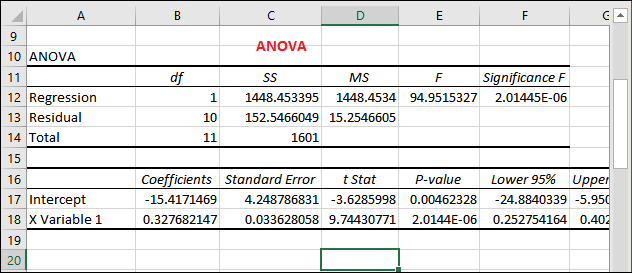
RESIDUAL OUTPUT

The last part is residual, which shows the difference between actual and estimated values. If you compare the results of both values for the total number of umbrellas sold each month, you will see that there will be a slight difference between both numbers.

If you will compare the actual umbrellas sold in January month and predicted value for it. You will get a slight difference in them.

Actual sold umbrella in January: 12

Predict value of sold umbrella in January: 9.486

The difference between the actual value and predicted value can be seen in residuals in their respective column.

12 – 9.486 = 2.514

You can match it under the RESIDUAL OUTPUT table.

Make a linear regression graph

You can also make a graph and plot the values on it to see the relationship between two variables. Thus, draw a linear regression chart.

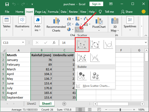
Step 1: Open your Sheet1 in the same Excel workbook and select the columns of independent variable and dependent variable along with the header.

Step 2: Navigate the Insert tab, where you see the chart group. Click on it, then choose Scatter (first one in the list). For easy to go, follow Insert > Chart group > Scatter.

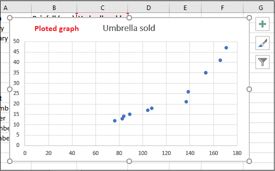
Step 3: A scatter plot chart will be inserted in your currently active workbook, which will look something like this –

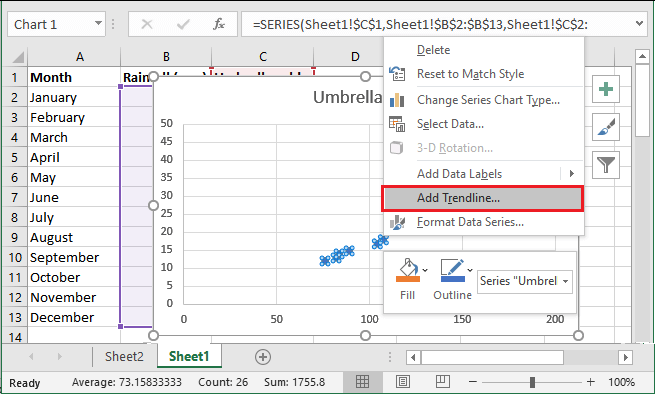
Step 4: Now, draw a least square regression line in this plotted chart. To do this, right-click on any of the points in this chart and choose Add Trendline? from the context menu.

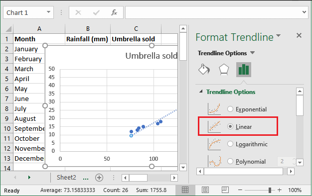
Step 5: Select the Linear trendline shape from the right side of the panel Format Trendline.

Step 6: Scroll down the format trendline panel and optionally mark the Display equation on chart to get the formula for regression. However, this one is optional.

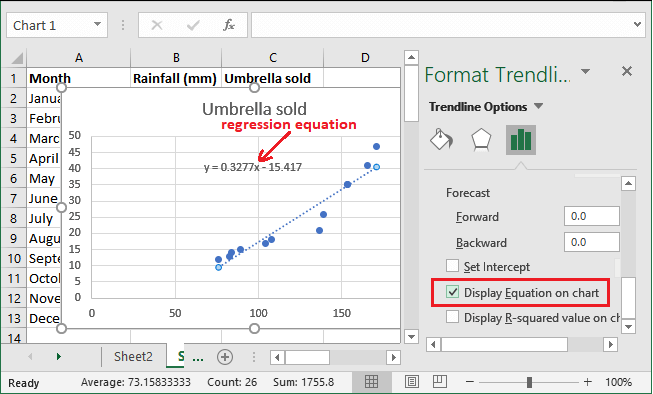
You can now see that the regression equation has been created.

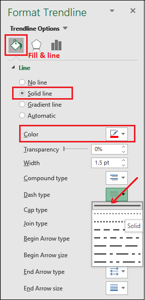
Step 7: Now, move to the Fill & Line option to customize the line you like. You can change the color and type of line from here. E.g., use a solid line instead of the dashed line.

• Firstly, Select the Solid line radio button, then scroll down.
• Change the line color to red or anything you want.
• Choose the solid line from the Dash type list.

See the customize linear regression graph.

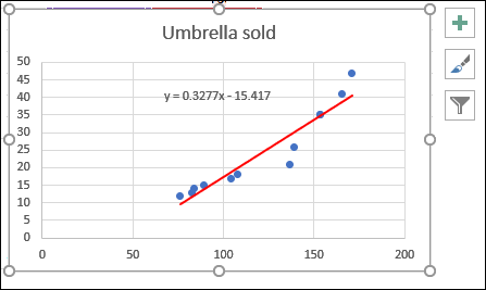
You can make some more improvements to the graph, like provide the axis title (horizontal and vertical) to the graph.