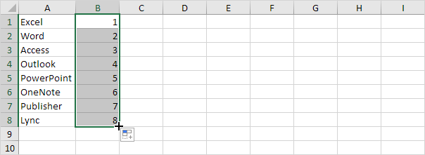
This article teaches you how to reverse a list in Excel. For example, we want to reverse the list in column A below.

1. Enter the value 1 into cell B1 and the value 2 into cell B2.

2. Select the range B1:B2, click the lower right corner of this range, and drag it down to cell B8.

3. Click any number in the list in column B.

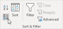
4. To sort in descending order, on the Data tab, in the Sort & Filter group, click ZA.

Result. Not only the list in column B, but also the list in column A has been reversed.