Excel Sorting: Master the Art with Abundant Examples

Sorting in Excel

To learn how to sort data need data. Let’s use the table below. 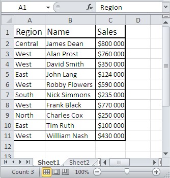You need sorting because that’s not look professionally. Sort sales descending.

Sorting starts marking data that you want to sort. In this case, select the range of cells A1: C11. Then go to the Data tab on the ribbon and press the Sort button. Dialog box appears. 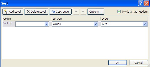Choose sort by Sales order Largest to Smallest value. Don’t forget to tick My data has headers check box. 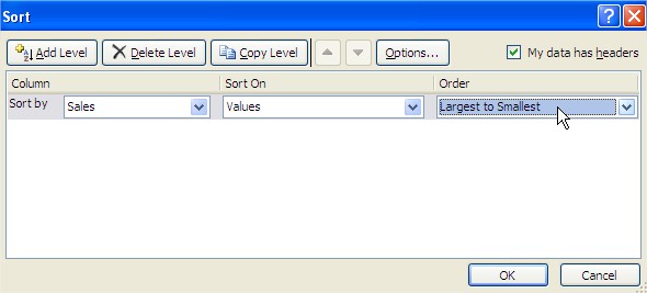You can also to add next level of sorting. Click Add Level and sort Regions alphabeticaly A to Z.

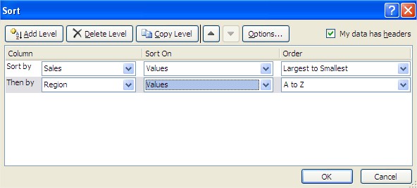
Sorting finished. Well done!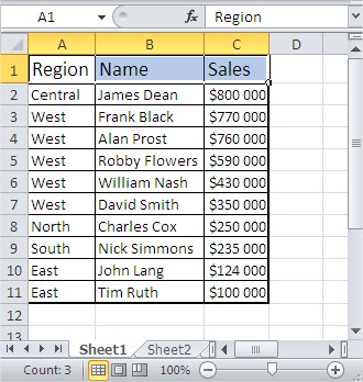

How to Sort by More than Three Columns?

The sorting of more than three columns can easily be performed. First you need a data that looks like this: 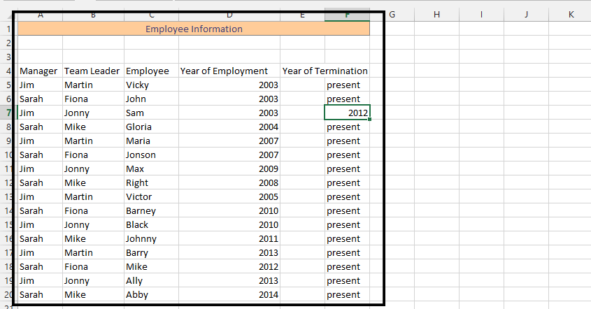1. Click on first cell of the data (manager). 2. Click on Data (1), and then press sort (2). 3. Choose “Year of Employment” in sort by, and then press ok. 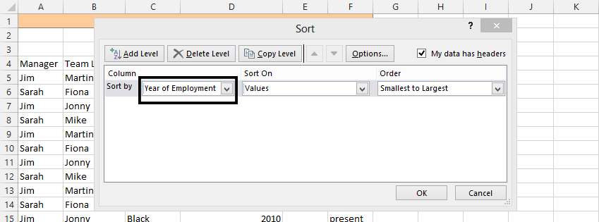4. Repeat, but in Sort by, choose manager (or the most important column) (1), and then click Add level (2), to choose the second most important column, and then press ok. 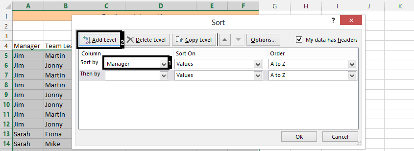Note: Keep repeating this step until you have sorted the columns from most important to least important. It is important to acknowledge that, if for instance cells in a column would exchange position for the sort to take effect, then Excel would ignore them.

After following the steps above, the sort would now look like this: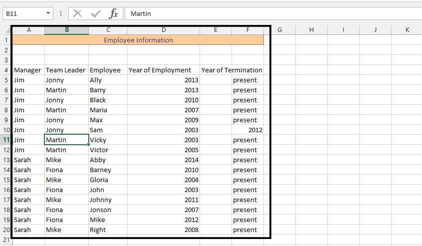

Sorting by color

You can also sort colors. You may need that especially when you like to color your spreadsheets like I do. I must admit it sometimes makes some problems in understanding the sheet but also gives me additional opportunieties.

To sort colours in your table first prepare colorful data table like this one in the picture below. 1. Click Data (1), and then click on sort (2). Note: You should first press the AZ beside the small picture showing ZA/AZ, so it makes easier to move ahead.

2. Choose the column (1), then choose color in sort by (2), and then order (3). 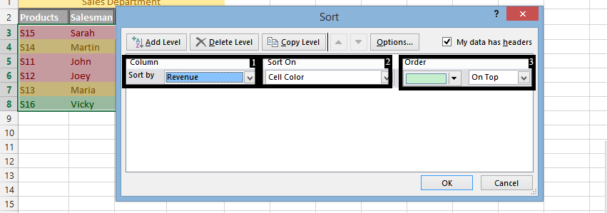Note: After following this step, press Add level, sorting by the same thing in column, cell color, and choose color you’d like to have on the second place. Continue until you’d add all the colors in the data, and then press ok.

How to Sort by Row?

Who said you need to sort only columns? Teach yourself how to sort by row. This trick maybe useful for large spreadsheets with many columns.

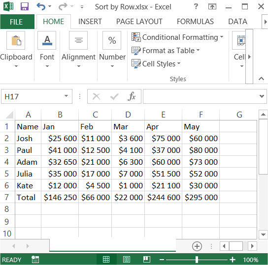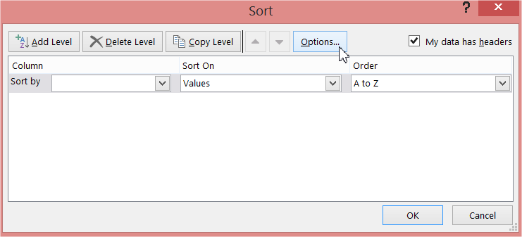
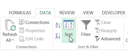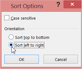
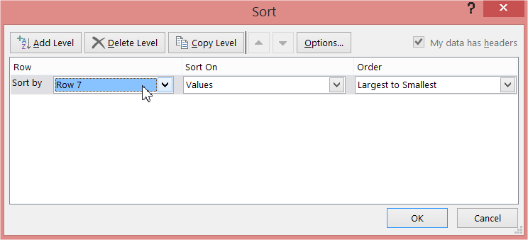
First prepare you data table. Here is an example. Go to the ribbon to the Data tab. Click Sort button. Sort dialog window appears. Click Options button. Click Sort left to right. Now decide what do you want to sort. I sorted Row7 (which is Total in my table) by Largest to Smallest order. Here you can see how Excel sorted the data. Total row is sorted descending. 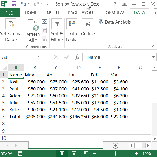This is how to sort by row within Excel.

Sorting a list of words by character count

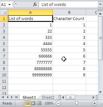
Excel lets to sort data not only alphabetically but also based on cell colour or font colour. Probably you didn’t know but you can also sort based on count of characters. To do this you will need some data. Let the picture below to be the example. 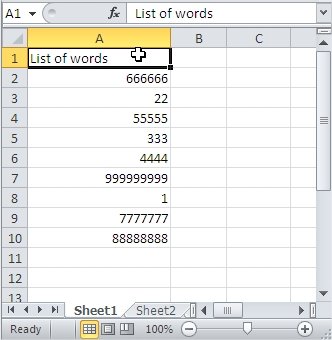In the B column write formula which refers to value in A column. In B2 formula will be: =LEN(A2) 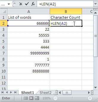Drag the formula down. 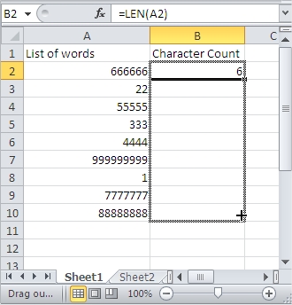Now you see count of characters of words in A column in B column. 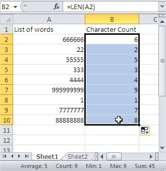Next highlight whole table and go to Ribbon > Data > Sort. Tick My data has headers and sort by Charcter Count Smallest to Largest. 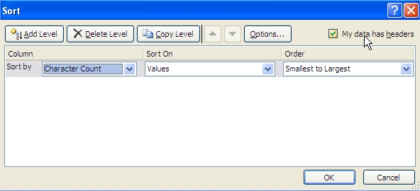Excel sorted your words from shortest to longest.

How to Sort Out Blank Rows?

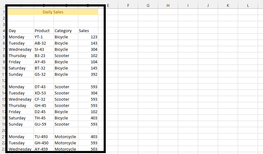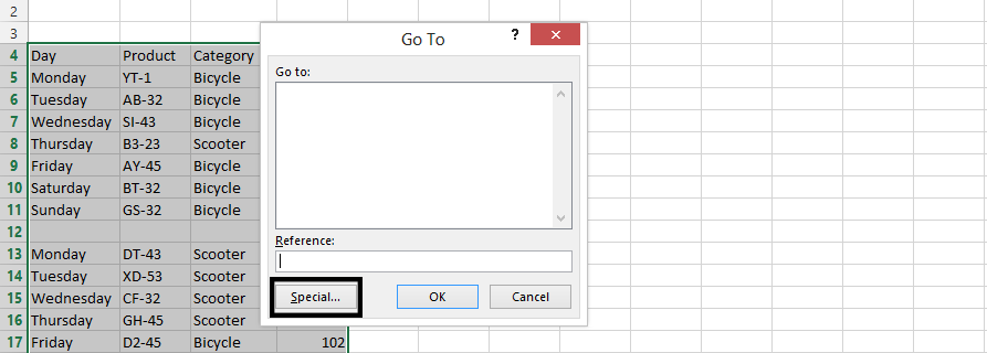
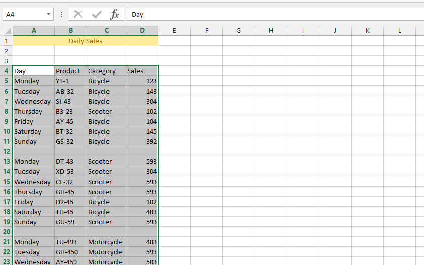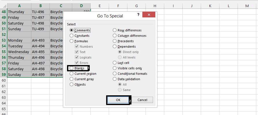
The sorting out blank rows comes down to one thing, how many they are, and that if they should be there or not. But first, have a look at this rows with both filled and empty rows: Mark the whole data. Press CTRL + G and click Special Choose Blanks Press Home (1), Choose a color with Cell Styles (2). Note: Give the blank cells a unique color. It is recommended that you’d use only one color in the actual data.

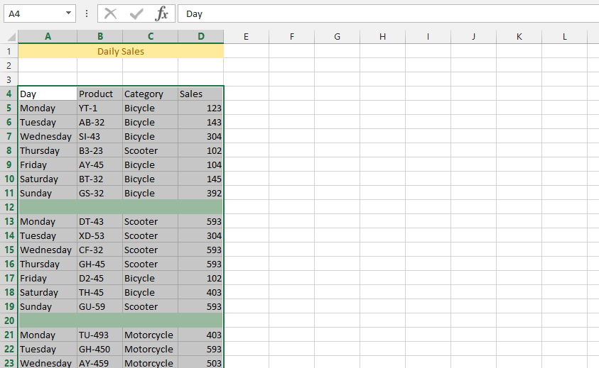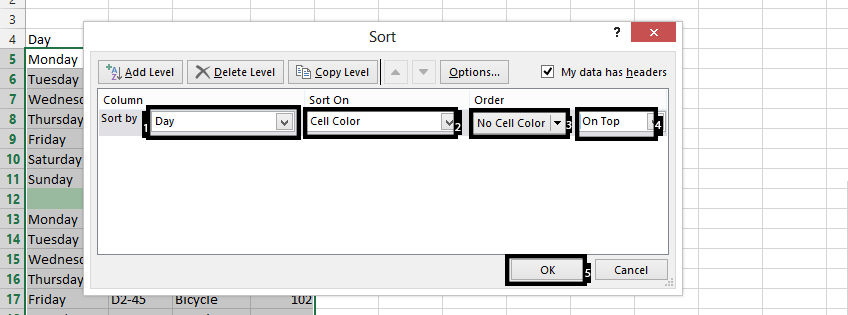
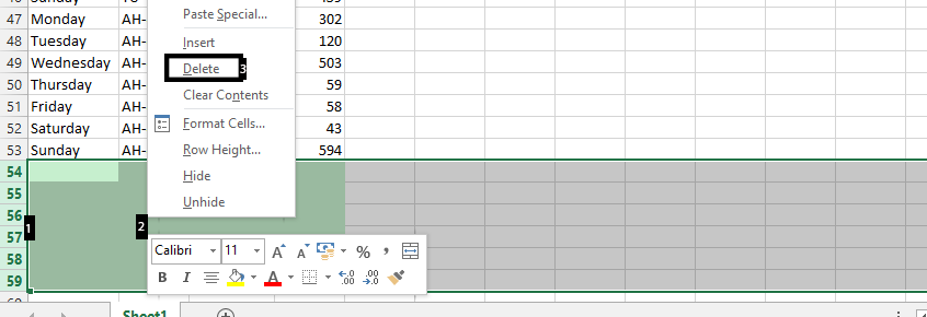
Mark the whole data again. Click on Data (1), and then on Sort (2). Choose a category in Sort by (1), choose cell color on Sort On (2), No Cell Color in order (3), On Top (4), and then press ok. Choose all the colored rows, right click on the marked rows (2), and choose delete (3).