

Sum Formula in Excel
Adding up data is one of the most popular activities in the Excel world. Because of this reason, Microsoft Excel is equipped with several built-in functions such as SUM, SUMIF, and SUMIFS. The built-in SUM function in Excel not only helps to sum up a range of cells, a row, column, or non-contiguous cells but can also be combined with other Excel functions to make advanced SUM formulas.
The tutorial, we will cover the various means to calculate the Sum Range, will determine the Sum of an entire column, the Sum of Non-contiguous cells, working with Excel AutoSum, steps to sum every Nth Row, how to calculate the Sum of the largest numbers, Sum Range with errors and many more.
Sum Range
This is one of the most commonly used operation in Excel. For most of the cases, users calculate the Sum Range using the built-in SUM function in Excel.
What is Sum Function?
The SUM function in Excel returns the sum of the specified range of cells. In any combination, these cells can contain numbers, cell references, ranges, arrays, and constants. The SUM function can accept up to 255 separate arguments.
Syntax
Parameters
number1 (required) – This parameter represents first value to sum.
number2 (optional) – This parameter represents second value to sum.
number3 (optional) – This parameter represents third value to sum.
Return value
The SUM function returns the sum of the given values.
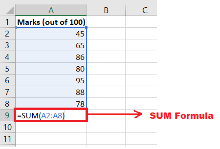
Example: Calculate the Sum Range for the given group of cells.
Following are the rules to quickly calculate the SUM Range using the SUM function:
- Select a cell where you will want the output of the Sum Range.
- If you want to calculate the sum of a column, select the cell below the last value in the same column.
- If you want to calculate the sum of a row, select the cell to the right of the last value in the same row.
- Start your formula with equal to ‘=’ and mention the SUM. In the arguments section, specify the range of cells for which you want to calculate the SUM. You can directly select the cells using your mouse cursor.
Formula becomes: = SUM (A4:A10)

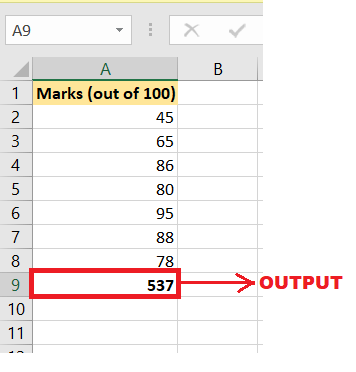
- Press the enter key once done. Excel will throw the following result:
Sum Entire Column
The SUM function can also be used to calculate the sum of an entire column.
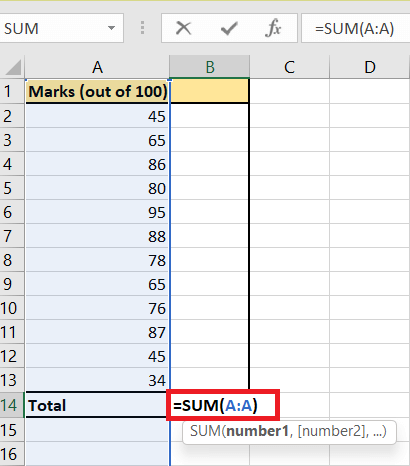
Example: Calculate the Sum of an entire column.
Following are the rules to quickly calculate the SUM of an entire column:
- Select a cell where you will want the output of the Sum Range.
- Start your formula with equal to ‘=’ and mention the SUM. In the arguments section, specify the column name for which you want to calculate the SUM. You can directly select the column using your mouse cursor.
Formula becomes: = SUM(A:A)
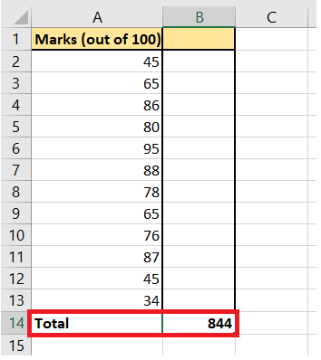
- Press the enter key once done. As a result, Excel will calculate the sum of entire column and fetch the following result:
NOTE: With some little changes you can use the above SUM function to calculate the sum of an entire row. For example, = SUM (10:10) adds all the cell values in the 10th row.
Sum Non-contiguous Cells
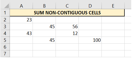
The term ‘Non-Contiguous’ refers to the cells that are not next to each other and are located at different positions on your worksheet. The SUM function in Excel can also calculate the sum of non-contiguous cells in your Excel spreadsheet.
Example: Calculate the Sum of the non-contiguous cells that contain numeric values.
Given-below are the steps to compute the SUM of the non-contiguous cells:
- Select a cell where you will want the sum output of the non-contiguous cells.
- Start your formula with equal to ‘=’ and mention the SUM. In the arguments section, you have to specify the individual cells.
Here’s a little trick.
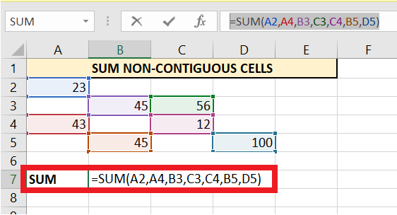
Press the CTRL button and using your mouse cursor click on the non-contiguous cells separately.
Formula becomes: =SUM(A2,A4,B3,C3,C4,B5,D5)
- Press the enter key once done. As a result, Excel will calculate the sum of the non-contiguous cells and will return the following output:
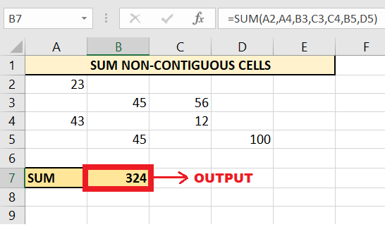
Note: Instead, you inserting the above formula, you can also calculate the sum with = A2 + A4 + B3 + C3 + C4 + B5 + D5. You will notice both the formula produces the exact same output!
SUM using AutoSum
Why manually enter the SUM formula and specify the range when Microsoft Excel can do the math for you. Whenever you want to calculate the sum of the range of cells, an entire column, row, or several adjacent columns or rows, you can rely upon the Excel AutoSum tool that automatically makes an accurate SUM formula. When you click AutoSum, Excel automatically create the SUM formula (using the inbuilt SUM function) to sum the specified cells.
To use Excel’s AutoSum tool, follow the below-given 3 steps:
STEP 1: Select the cell
Select a cell where you will want the sum output of the AutoSum
- If you want to calculate the sum of a column, select the cell below the last value in the same column.
- If you want to calculate the sum of a row, select the cell to the right of the last value in the same row.
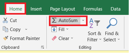
STEP 2: Click on AutoSum
Go to the Home tab. Click on the Editing group > AutoSum:
OR
Click on the Formulas tab. Go to the Function Library group > AutoSum:
You will notice that a Sum formula will appear in the selected cell, and the cells that you want to add will get highlighted (A2:A13 in this example):
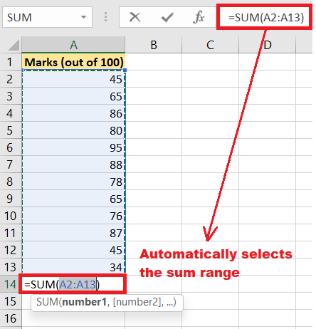
Though in most of the cases, Excel automatically selects the accurate range of cells that you want to SUM. But in some case, there are chances if you choose a wrong selection, but you can correct it manually by typing the preferred range in the formula bar or by dragging the mouse cursor through the cells you want to sum.
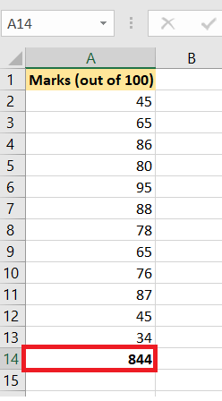
STEP 3: Press the Enter button to complete the process.
Now, you can see the calculated total in the cell, and the SUM formula in the formula bar:
NOTE: If you one of those Excel users who prefer working with the keyboard rather than the mouse, you can use the following Excel AutoSum keyboard shortcut to total cells:
press ‘ALT’ + ‘=’ to quickly sum a column or row of numbers.
Sum Every Nth Row
In some cases, however, we are only required to sum a specific range of cells in an excel worksheet, say the sum of every 3rd row, to 6 to sum every 7th row, etc. Some users may find it challenging because Microsoft Excel doesn’t contain any built-in function to calculate this. But as always, Excel formulas are the saviour since nothing can prevent you from creating your customised formulas!
To find the Sum of every Nth Row we can use the combination of the Excel functions like SUM, MOD and ROW. Given-below are the steps to compute the SUM of every Nth row:
- Select a cell where you will want the sum output of every Nth row.
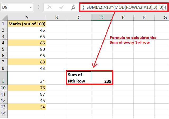
- Start your formula with equal to ‘=’ and mention the SUM. To calculate the sum of every 3rd row, we will create a formula using the combination of SUM, MOD and ROW functions.
Formula becomes: {=SUM (A2:A13*(MOD(ROW(A2:A13),3)=0))} - Press the enter key once done. As a result, Excel will calculate the sum of the non-contiguous cells and will return the following output:
- If you want to calculate the sum of every 5th row, simply change the 3 to 4 to sum every 5th row.
Note: In the above formula, you will notice that we have put the formula in curly braces {}. These braces indicate that it is an array formula. But always remember not to type them manually. Enter an array formula to the above formula by pressing the keyboard shortcut CTRL + SHIFT + ENTER.
Sum Largest Numbers
If you store business data in Excel, such as sales data for a specific region, the weight of certain machinery parts, and expenses of a month, you may need a quick way to sum up, the largest numbers to prices or amounts.
Below are very simple and straightforward steps to calculate the SUM of the largest numbers in a range using the inbuilt SUM and LARGE. Even if you are a beginner in Excel, you will hardly have any problem understanding the following examples.
- Select a cell where you will want the output of the Sum of largest numbers Range.
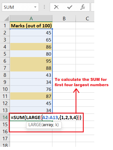
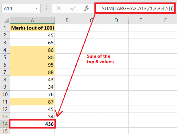
- Start your formula with equal to ‘=’ and mention the SUM. In the arguments section, specify the LARGE function, inside the parameters mention range of cells for which you want to calculate the SUM and in the ‘k’ parameter specify the array values {1,2,3,4} since we have to calculate the top 4 values.
Formula becomes: =SUM(LARGE(A2:A13,{1,2,3,4}))
- Press the enter key once done. Excel will return the following result:
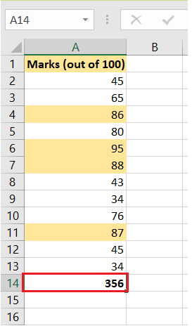
- If you want to find the sum of 5 largest number simply change {1,2,3,4} to {1,2,3,4,5}.
Note: With a little modification you can also calculate second largest number using the formula =LARGE(A1:A11,2).
Sum Range with Errors
Formula and Error run hand in hand. Similarly, while working with the sum formula, users often end up with Excel errors.
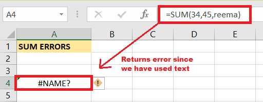
In the below image, as you can see the SUM formula returns the #NAME? error since we have incorporated text within the formula.
Using error control methods can check the errors. A combination of the inbuilt SUM and IFERROR functions is used to sum a range with errors. You can also use the AGGREGATE function in Excel to sum a range with errors.
Following are the rules to quickly calculate the SUM Range using the SUM function:
- Select a cell where you will want the output of the Sum Range.
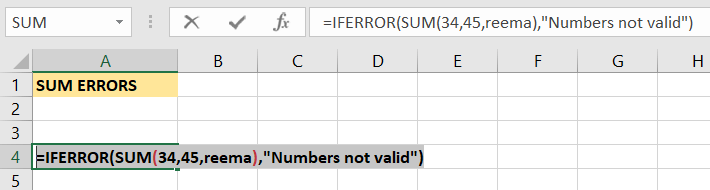
- Start your formula with equal to ‘=’ and mention the IFERROR function to check if there exists any error. In the value arguments, we will specify the SUM function and the values. In the value_if_error argument of the IFERROR function, we will specify the text you want to display instead of the error. You can directly select the cells using your mouse cursor.
Formula becomes: =IFERROR(SUM(34,45,reema),”Numbers not valid”)
NOTE: You can also enter customised message in the IFERROR function. - Press the enter key once done. Instead of throwing the error, Excel will return the IFERROR text. You will have the following result:
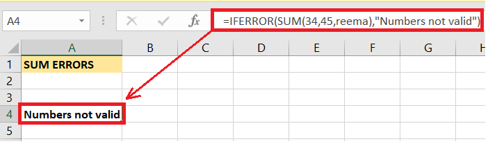
NOTE: The Excel SUM function automatically ignores the text values.
Eureka! Now since we have covered all the SUM topics. Go ahead and create great SUM formulas per your requirement and shine like a star among your colleagues.


