Trend Function Excel
In today’s technology-driven world, markets and customer needs are changing so rapidly that it is essential that you move with trends and not against them. Trend analyses are very useful since they help look for the underlying patterns in the past and present data actions and predict future project behavior.
In this tutorial, you will learn what the Trend function is, its syntax, parameter, points to remember, how this formula works, and various examples by using the TREND function to calculate the linear trend `on the basis of the specified linear data set.
What is Trend Function in Excel?
“The Trend is an inbuilt Statistical function in Excel that calculates the linear Trend on the basis of the specified linear data set. This function is used to calculate the predictive values of Y for a certain array value of X and uses the least square method on the basis of the given set of data series.“
The Trend function in Excel returns numbers in a linear trend matching known data points, that is, the existing data on which the trend forecasts the values of dependent Y (known y’s parameter) on values of X (that needs to be present in linear data format).
What is the least square method?
Least Square Method is an useful Excel technique used in the regression analysis that searches the line of best fit (is a line through a scatter graph of data points that foremost indicates the relationship between those points) for a specified set of data, which helps to envision the connection between the different data points.
How TREND function calculates linear trendline
The Excel TREND Function finds the line that best fits your data using the least-squares method (explained above). The equation for the line is given below:
As per the least squares method, equation to represent one range of x values:
As per least squares method, equation to represent multiple ranges of x values:
Where:
y – The axis y is dependent upon the variable the user wishes to calculate.
x – The axis x is independent of the variable that the user is using to calculate y.
a – It represents the intercept (specifies where the given line intersects the y-axis and is equal to the value of y where the value of axis x is 0).
b – It represents the slope (specifies the steepness of the line).
Syntax
Parameter
Known_y’s (required) – This argument represents a given set of the dependent data values of the y-axis that the user already knows.
Known_x’s (optional) – This argument accepts one or more sets of the independent x-values.
- If the user is using only one x variable, the parameters known_y’s and known_x’s can form ranges of any shape but of equal dimension.
- If the user is defining several x variables, the parameter known_y’s should be a vector (one column or one row).
- If the parameter known_x’s is omitted, by default, it is assumed to be the array of serial numbers {1,2,3,…}.
New_x’s (optional) – This argument represents one or more new x-values for which the user wants to calculate the trend.
- New_x’s argument must contain the equal number of columns or rows as used for known_x’s parameter.
- If the user doesn’t mention this parameter, by default, it is equal to the known_x’s parameter.
Const (optional) – This parameter represents a logical value specifying how the constant value in the equation y = bx + a should be computed.
- If the user specifies TRUE or if this parameter is omitted, the constant value is computed normally.
- If the user specifies FALSE, the value for constant a is forced to be equal to 0, and the b-values are adjusted to fit the equation y = bx.
Return Type
The Trend function in Excel returns numbers in a linear trend matching based on the specified linear data set.
#Trend Example 1: Predict the GPA for given values using TREND function.
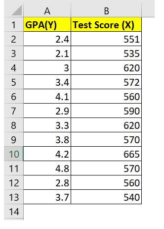
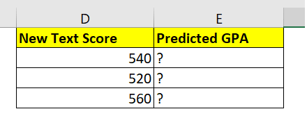
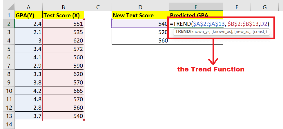
In this example, as you can see in the below table, we are given data for different test scores with their GPA. Predict the GPA value for different data. We already have data in columns A and B of the above table. We will interpret the existing values of GPA as the Y values, and their corresponding text scores are the known values of Y. We already have some values for X values as a score. Below we are given some new text scores for which we have to calculate the new GPA based on the existing values.
Predict the GPA values
We will use the inbuilt Trend function to predict the above GPA values. Follow the below-given steps to compute the GPA for the above series of data flows using the Excel TREND () function:
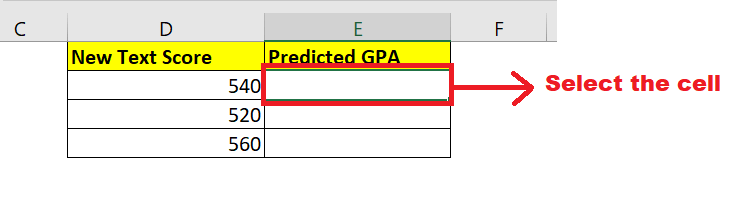
Step 1: Select a cell to calculate TREND
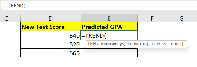
Place your mouse cursor to a cell from where you want to have the TREND() function result. Since we have to look for the GPA for cell E2, we have selected cell E2 to type our function.
Refer to the given below image:
STEP 2: Type the TREND function
In E6, we will start typing the function with the equal to (=) sign followed by the TREND function. The function becomes: = TREND(
STEP 3: Insert all the parameters
- The TREND formula in excel will ask you to specify the known_ys parameter. For this argument we will take the existing range of known Y values. The formula will become: =TREND($A$2:$A$13,
NOTE: We have used absolute reference for the above range of values because we want to keep them fixed while using the formula for the next cells.
- Next, for option known_xs argument, we will specify the text score values of X to calculate the values for GPA in cell E2, E3, and E4. The formula will become: =TREND($A$2:$A$13, $B$2:$B$13,
NOTE: Since, we want to keep this value fixed, we have used the absolute reference for this parameter as well
- Next, we will specify the new text score. The overall formula becomes: =TREND($A$2:$A$13, $B$2:$B$13,D2)
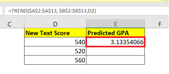
Step 4: The TREND function will return the output
As a result, the TREND function will return the predicted GPA for the given new text score on the basis of the earlier patterns of X and y data ranges.
Step 5: Drag and Repeat the function to other cells
Select the formula cell and drag the cursor towards the right corner of the rectangular box. You will notice that your cursor will change into a plus (+) icon.
Drag the icon to the below two cells, and the formula will be replicated to all the cells changing the respective values accordingly where the absolute references will remain fixed.
You will have the following output.
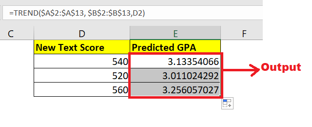
So, using the Excel TREND function, we predicted the three values of Y for the specified new test scores.
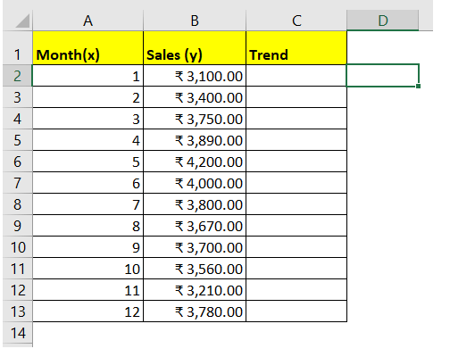
#TREND Example 2: Analyse the given data for a sequential period of time, spot the trend.
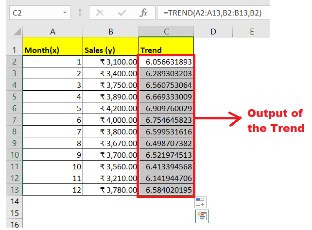
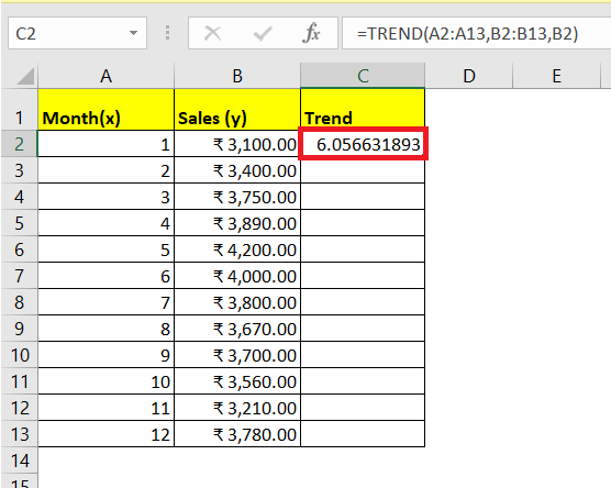
Let’s solve another example so you can understand the behavior Trend function, and then this function might seem less complicated to you. In this example, we are given the month numbers (representing the x-values) in column A and sales numbers (representing the dependent y-values) in column B.
Based on this data, we will find the overall trend in the time series overlooking hills and valleys.
We will use the inbuilt Trend function to spot the trend. Follow the below-given steps to compute the GPA for the above series of data flows using the Excel TREND () function:
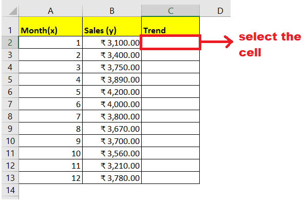
Step 1: Select a cell to calculate TREND
Place your mouse cursor to a cell from where you want to have the TREND() function result. Since we have to look for the GPA for cell E2, we have selected cell E2 to type our function.
Refer to the given below image:
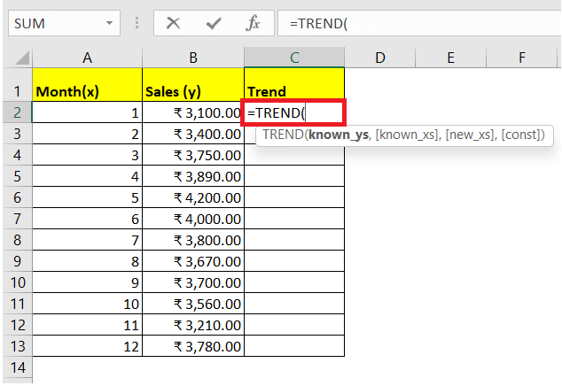
STEP 2: Type the TREND function
In E6, we will start typing the function with the equal to (=) sign followed by the TREND function. The function becomes: = TREND(
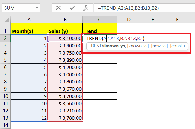
STEP 3: Insert all the parameters
- The TREND formula in excel will ask you to specify the known_ys parameter. For this argument we will take the existing range of known Y values. The formula will become: =TREND($A$2:$A$13,
NOTE: We have used absolute reference for the above range of values because we want to keep them fixed while using the formula for the next cells.
- Next, for option known_xs argument, we will specify the text score values of X to calculate the values for GPA in cell E2, E3, and E4. The formula will become: =TREND($A$2:$A$13, $B$2:$B$13,
NOTE: Since, we want to keep this value fixed, we have used the absolute reference for this parameter as well
- In the next parameter, specify the sales of the x axis. The formula will become: =TREND($A$2:$A$13, $B$2:$B$13,B2)
Step 4: The TREND function will return the output
As a result, the TREND function will return the predicted GPA for the given new text score on the basis of the earlier patterns of X and y data ranges.
Step 5: Drag and Repeat the function to other cells
Select the formula cell and drag the cursor towards the right corner of the rectangular box. You will notice that your cursor will change into a plus (+) icon.
Drag the icon to the below two cells, and the formula will be replicated to all the cells changing the respective values accordingly where the absolute references will remain fixed.
You will have the following output.