Types of References in Excel
A worksheet in Excel is made up of cells. These cells can be referenced by specifying the row value and the column value. In Excel, a cell reference is a technique to signify any cell’s identity and location by combining column names and row numbers on a worksheet. For example, suppose we say A5, then it expands as a column A and 5th Row. Similarly, we can also declare or define cell references to any location in the worksheet. We may also activate R1C1 from Excel options, which is another means of referencing cells, with R1 denoting Row 1 and C1 denoting Column 1.
Types of Cell Reference in Excel
The following are the three types of references in Excel:
- Relative cell references
- Absolute cell references
- Mixed cell references in Excel
1. Relative Cell References
In Excel, a relative reference is a form of a cell reference. By default, all cell references are relative references. Relative references are changed when copied across different cells based on the relative positions of rows and columns. For example, suppose we copy the formula =B1*C1 from row 1 to row 2, the formula will become=B2*C2. When we have to repeat a calculation across numerous rows or columns, relative references are extremely useful.
2. Absolute Cell References
In Excel, an absolute cell reference is one of the cell reference types in which the cells being referred to do not alter like they did in a relative reference. We utilize the $ sign by pressing f4 to create a formula for absolute referencing. The $ sign means lock, and it locks the cell reference for all of the formulas, ensuring that the same cell is referred to all of them.
3. Mixed Cell Reference in Excel
A Mixed cell reference is a mixture of both relative and absolute cell reference. In mixed cell reference, dollar signs are attached to either the letter or the number. For example, $B2 or B$4. It’s a mix of relative as well as absolute reference.
Let’s take a closer look at each of the cell references:
How to Use Relative Cell Reference?
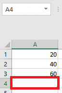
Example 1: Let’s look at a basic example to demonstrate how Relative Reference works in Excel. Suppose we want to multiply three numbers in three different cells-A1, A2 and A3, and the result in the third cell-A4.
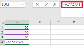
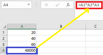
So, we use the formula A1*A2*A3, which gives us 48000 in cell A4.
The result is 48000
Assume that the next column (“B”) contains a similar circumstance. Cell B1, B2, and B3 have three numbers, and we want to have the multiplication in B4.
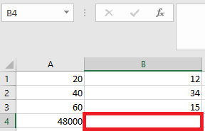
By using two ways, we can achieve this:
In the first way, we can manually write the formula to multiply B1, B2, and B3 in order to obtain the result.
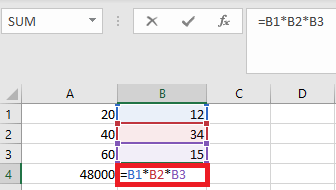
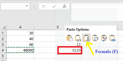
The result is 6120
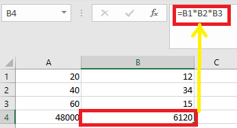
Another way is we can easily copy the formula from cell A4 and paste it into cell B4.
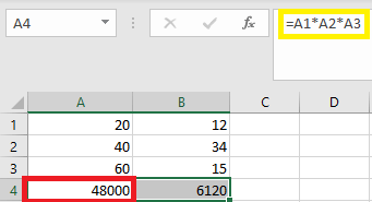
As a result, when we copy the value of the A4 cell and paste it in B4 or drag the content of A4 and paste in B4, only the formula is copied, not the result. By right-clicking on cell A4 and selecting Copy, we may achieve the same outcome.
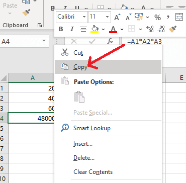
Then, we move to the next cell, B4, and right-click, and select “Formula (f)” from the paste options.
Example 2: With the help of this example, we will discuss more about the use of the relative cell reference. In this example, we have a Pharma Sales table; a table contains medicine products in column A (A2:A7), quantity sold in column B (B2:B7), price in column C(C2:C7), and Total sales value in Column D, that we need to determine.
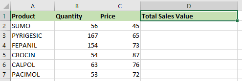
If we want to compute the total sales for each item, we have to multiply the price of each product by the quantity of that item.
Consider the first item; the formula in cell D1 for the first item would be multiplication in Excel=B2*C2.
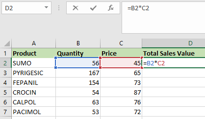
The above formula will return the total sales value.
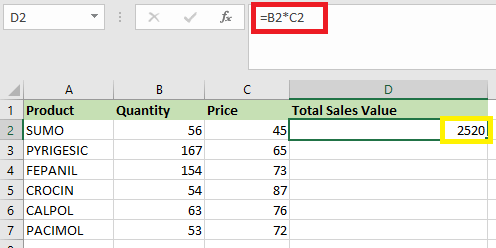
We may now apply the formula to the entire range rather than typing it for each cell individually. In order to copy the formula down the column, we need to click inside cell D2, and we will see the cell selected, select the cells up to D7. As a result, that column range will be selected. After that, use Ctrl+D in order to apply the formula to the entire range.
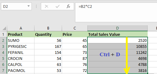
Here, when we copy or move a formula with a relative cell reference to a different row, the row references will update automatically (similarly for columns also).
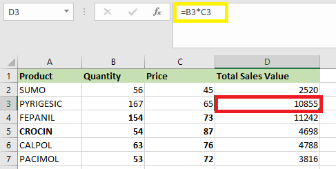
The cell reference immediately adjusts to the correct row, as we can see or notice above.
In order to examine a relative reference, we have to select any of the cells of the Total sales value in Column D, and the formula will appear in the formula bar. For instance, in cell D3, the formula has changed from =B2*C2 to =B3*C3.
When to Use Relative Cell References in Excel?
Relative cell references are helpful when we need to create a formula for a range of cells, and the formula needs to refer to a relative cell reference. In such situations, we can make the formula for one cell and then copy-paste it into others.
How to Use Absolute Cell References in Excel?
With the help of the following example, we will discuss about the use of the absolute cell reference.
The use of absolute cell references is seen in the table below:
| Absolute Reference | Particular | Keys in the Keyboard |
|---|---|---|
| $A1 | When we copy a column, it stays the same. | Press F4 three times. |
| $A$1 | When we copy a column or a row, nothing changes. | Press F4. |
| A$1 | When we copy a row, it stays the same. | Press F4 twice. |
When writing formulas with absolute references, we will usually use the $A$1 syntax. The other two formats are used much less frequently.
We can switch between relative and absolute cell references by pressing the F4 key on our keyboard while creating a formula. This is a quick and simple technique to insert an absolute reference.
Absolute cell references do not alter when the formula is copied to other cells, unlike relative cell references.
Example 1:
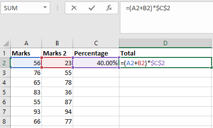
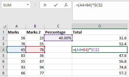
- We write the formula in any cell, and then we have to press the enter to calculate it. In this example, we used the formula =(A2+B2)*$C$2) in cell D2 and press Enter to calculate the formula.

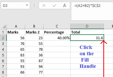
- Next, we have to click on the Fill handle at the cell’s corner that comprises the formula (D2).

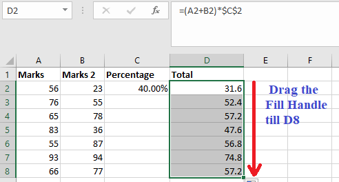
- Now, we drag the fill handle up to the cells which we want to fill. In this example, we will drag it to cell

- Now, the percentage is calculated in column D, as we can see in the below screenshot.

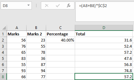
- We may double-click any cell to examine which cells the operation is performed, and we see that cell C2’s address remains unchanged.

As we can see in the previous example, the address of cell C2 remains the same while the addresses of columns A and B vary in response to the relative position of the row and column. This is because we used the absolute address of cell C2.
Example 2:
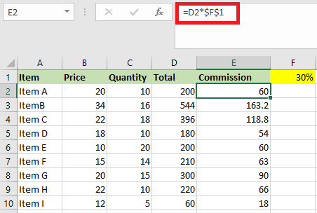
Suppose we have the following data set and need to determine the commission for each item’s total sales.
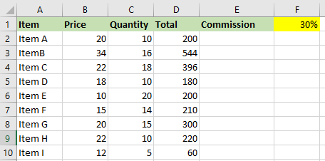
30% is the commission that is listed in cell F1.
To calculate the commission amount for each item sale, we have to enter the following formula in cell E2 and copy it to all other cells.
What does the Dollar ($) sign do?
When the dollar symbol is placed in front of the row and column number, the cell becomes absolute (means it stops the row and column number from changing when copied to other cells).
For example, in the above case, if we copy the formula form E2 to E3, it modifies from =D2*$F$1 to =D3*$F$1.
It’s worth noting that, while D2 changes to D3, $F$1 remains unchanged.
Because we put a dollar symbol in front of ‘F’ and ‘1’ in F1, the cell reference would not be changed when we copied it.
As a result, the cell reference is now absolute.
When to Use Absolute Cell References in Excel?
We used absolute cell reference when we don’t need the cell reference to modify when copying the formulas from one cell to another. This could be the situation when we have a fixed value which we have to utilize in the formula (like commission rate, tax rate, number of months, etc.).
While we could hard code this amount in the formula (e.g., $F$2 instead of 30%), putting it in a cell and then utilising the cell reference allows us to alter it afterward.
For example, if our commission structure changes and we are now paying 30% instead of 25%, we can just modify the number in cell F2, and all the calculations will update instantly.
How to Use Mixed Cell References in Excel?
Absolute and relative cell references are easier to work with than mixed cell reference, whereas mixed cell references are more difficult.
There are two types of mixed cell references:
- The row is locked while the column changes when the formula is copied.
- The column is locked while the column changes when the formula is copied.
Consider the following example to illustrate how it works:
Example 1: The following example demonstrates how to use both forms of mixed references in practices.
In the below table, we have a list of products along with their prices. For each product, there are two types of discounts.
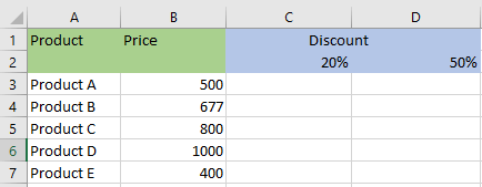
We have to enter the following formula into cell C3.
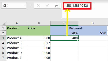
The formula is locked on column B ($B3) and row 2 (C$2).
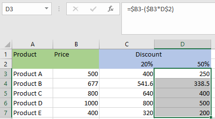
If we need to autofill the cell which is below the (C4) cell, then Excel will pick the next row for the Price ($B4) but not the row for (C$2) therefore, this column will always have a 20% discount.
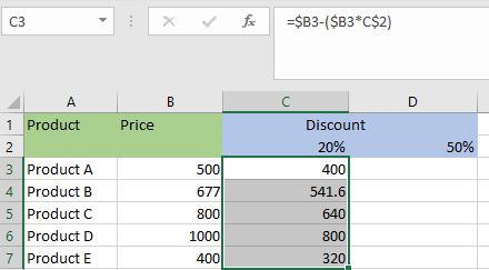
Let’s see how it works for the cell right, which is D3. Column B ($B3) will not change because it is locked.
The cell C$2 will change to D$2 because there is no lock on the column, only the row. Because we are in the same row in this example, the D3 formula is as follows:
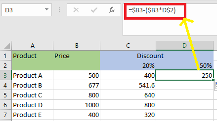
After we fill the remaining cell, we will get the below result:
Example 2: Below is the data set, and we have to calculate the three tiers of commission based on the percentage value in cells E2, F2, and G2.
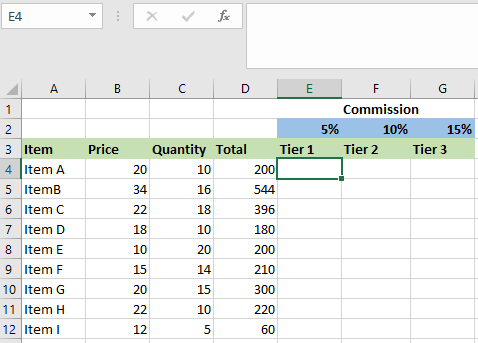
Now we can use the power of the mixed reference to compute all of these commissions with a single formula.
We will type the following formula in the cell E4 and copy all cells:
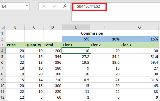
In this calculation above, both forms of mixed cell references are used (one where the lock is locked and one where the column is locked).
Let’s take a look at each cell reference and see how it works:
- $B4 (and $C4): – The dollar sign appears immediately before the column notation but not before the Row number. Because the column is fixed, the reference will remain the same when we copy the formula to the cells on the right. For example, if we copy the formula from E4 to F4, this reference would not change. However, because it is not locked, the row number will vary when we copy it down.
- E$2: – The dollar sign comes exactly before the row number in this reference, although the column notation does not include a dollar sign. This implies that when we copy the formula down the cells, the reference will not change as the row number is locked. However, because the formula is not locked, the column alphabet will change if we copy the formula to the right.
How to Change the Reference from Relative to Absolute (or Mixed)?
If we wish to modify the reference from relative to absolute, we must place a dollar sign before the column notation and row number. For example, A1 is a relative cell reference, but when we change it to $A$1, it becomes absolute.
If we only need to modify a number of references, we may find it simple to do so manually. As a result, we can either alter the formula in the formula bar) or select the cell, press F2, and then change it).
However, utilising the keyboard shortcut-F4- is a faster way to achieve this.
When we press F4 while selecting a cell reference (in the formula bar or edit mode), the reference is changed.
If we have the reference=A1 in a cell.
When we choose the reference and press the F4 key, this is what occurs.
- Press F4 key once: The cell reference changes from A1 to $A$1(becomes ‘absolute’ from ‘relative’).
- Press F4 key two times: The cell reference changes from A1 to A$1 (changes to missed reference where the row is locked).
- Press F4 key three times: The cell reference changes from A1 to $A1 (changes to mixed reference where the column is locked).
- Press F4 key four times: The cell reference becomes A1 again.


