Remove Duplicates
This example teaches you how to remove duplicates in Excel.
1. Click any single cell inside the data set.
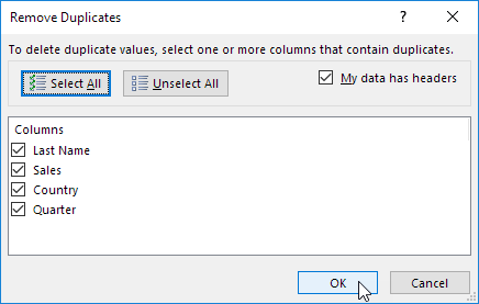
2. On the Data tab, in the Data Tools group, click Remove Duplicates.

The following dialog box appears.
3. Leave all check boxes checked and click OK.
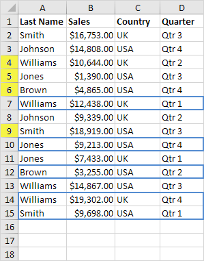
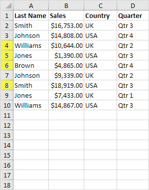
Result. Excel removes all identical rows (blue) except for the first identical row found (yellow).


To remove rows with the same values in certain columns, execute the following steps.
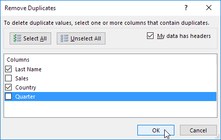
4. For example, remove rows with the same Last Name and Country.
5. Check Last Name and Country and click OK.
Result. Excel removes all rows with the same Last Name and Country (blue) except for the first instances found (yellow).
Let’s take a look at one more cool Excel feature that removes duplicates. You can use the Advanced Filter to extract unique rows (or unique values in a column).
6. On the Data tab, in the Sort & Filter group, click Advanced.

The Advanced Filter dialog box appears.
7. Click Copy to another location.
8. Click in the List range box and select the range A1:A17 (see images below).
9. Click in the Copy to box and select cell F1 (see images below).
10. Check Unique records only.

11. Click OK.
Result. Excel removes all duplicate last names and sends the result to column F.
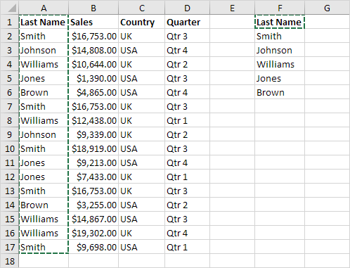
Note: at step 8, instead of selecting the range A1:A17, select the range A1:D17 to extract unique rows.
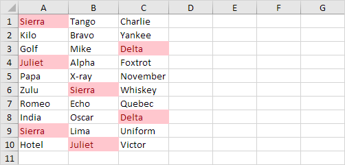
12. Finally, you can use conditional formatting in Excel to highlight duplicate values.
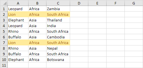
13. Or use conditional formatting in Excel to highlight duplicate rows.
Tip: visit our page about finding duplicates to learn more about these tricks.
Next Chapter: Conditional Formatting


