By default, the VLOOKUP function performs a case-insensitive lookup. However, you can use INDEX, MATCH and EXACT in Excel to perform a case-sensitive lookup.

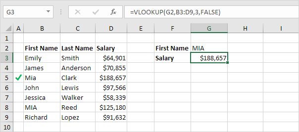
1. For example, the simple VLOOKUP function below returns the salary of Mia Clark. However, we want to lookup the salary of MIA Reed (see cell G2).

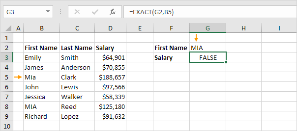
2. The EXACT function in Excel returns TRUE if two strings are exactly the same. The EXACT function below returns FALSE.

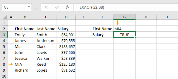
3. The EXACT function below returns TRUE.

4. Replace B8 with B3:B9.

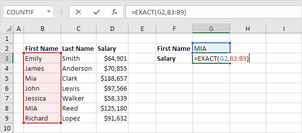
Explanation: The range (array constant) created by the EXACT function is stored in Excel’s memory, not in a range. The array constant looks as follows:

{FALSE;FALSE;FALSE;FALSE;FALSE;TRUE;FALSE}

5. All we need is a function that finds the position of TRUE in this array constant. MATCH function to the rescue! Finish by pressing CTRL + SHIFT + ENTER.

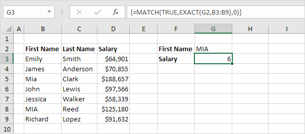
Explanation: TRUE (first argument) found at position 6 in the array constant (second argument). In this example, we use the MATCH function to return an exact match so we set the third argument to 0. The formula bar indicates that this is an array formula by enclosing it in curly braces {}. Do not type these yourself.

6. Use the INDEX function (two arguments) to return a specific value in a one-dimensional range. In this example, the salary at position 6 (second argument) in the range D3:D9 (first argument).

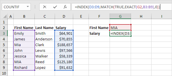
7. Finish by pressing CTRL + SHIFT + ENTER.

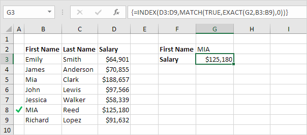
Note: the formula correctly looks up the salary of MIA Reed, not Mia Clark. The formula bar indicates that this is an array formula by enclosing it in curly braces {}.