How To Insert Waffle Chart In Excel
To start preparing Waffle Chart in Excel you need to prepare chart area. I did it for 10 x 10 cells area what is the most used for that type of chart. As you see on the picture below I set grey color for cells background and also changed font color for grey. It is important to use the same color.
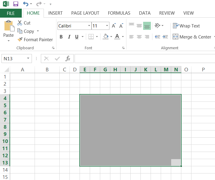
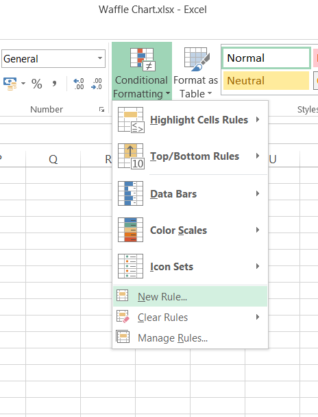
Next you need to set conditional formatting for cells inside chart area. To do it go to ribbon and click Conditional Formatting -> New Rule.
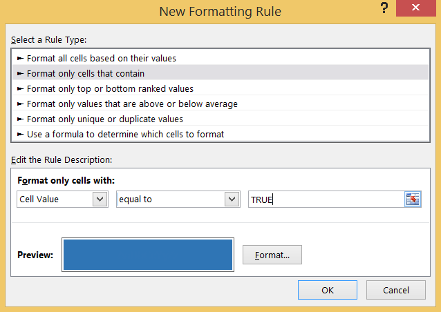
New Formatting Rule should be set for cells that contain equal to TRUE value. Also you need to click Format button and set Font color and Fill to the same color. I chose blue.
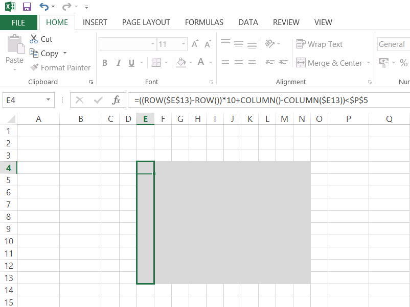
Next click the first cell in your chart area and use this formula:
=((ROW($E$13)-ROW())*10+COLUMN()-COLUMN($E13))<$P$5
Drag and drop the cell and set it for every cell in the whole area.
The last step is the value. Type some value to the P5 cell to check if the Waffle Chart is working properly.
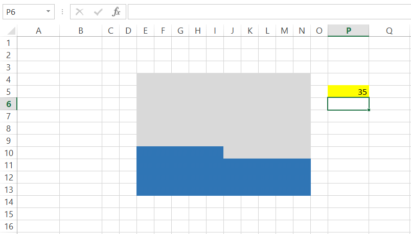
In the end you can to format you chart. It can look like this…
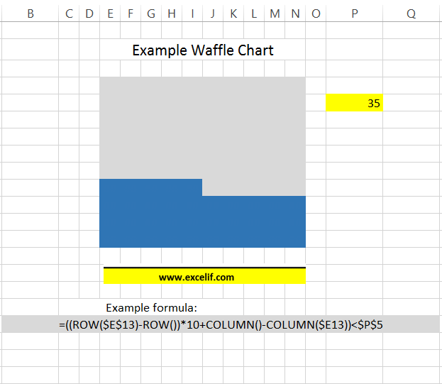
…or your chart can be more fancy like this one.
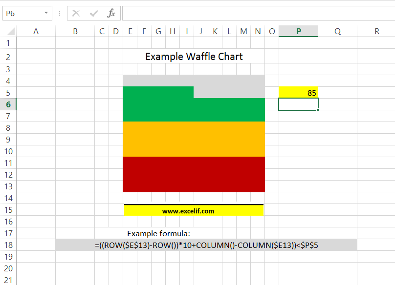
Template
Further reading:
Basic concepts
Getting started with Excel
Cell References


