Excel Array Formulas: Powerful Multicell Calculations

When an array formula, and when the regular?

An array formula (entered as an array) you use wherever you want to make a feature that “every day” operates on a single value (cell), suddenly behaved differently, and adopted as an argument and returned as a result of an array of values. Returning to the aforementioned IF function. As an argument it accepts a Boolean value of TRUE or FALSE. In the classic form:

=IF($B$7>”bigger”,”smaller”)

if the value in cell B7 is greater than zero, the function receives as an argument to TRUE and returns a string result “bigger”. However, if you wanted to see more single cells and the outcome of such consultations pass to yet another feature you should use the array version of the below formula:

{=IF($B$7:$B$10>”bigger”,”smaller”)}

Function takes as argument the whole range $B$7: $B$10 The examination of each cell in the memory array is formed

{TRUE, FALSE, TRUE, TRUE}

Then, we create another array, whose values depend directly on values in the first array. If in the first array element is TRUE, the second array will be set to “bigger”. If it is set to FALSE in the second array element takes the value “smaller”. After this operation, the first array is removed from the computer’s memory and, ultimately, the function returns the following array {“bigger”, “smaller”, “bigger”, “bigger”}.

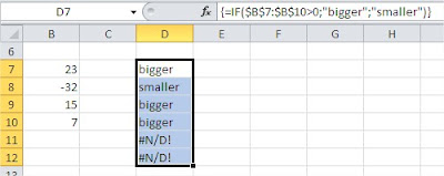
In my example, I entered an array formula to one cell (as seen in the picture above), so as a result I received only a single value corresponding to the first value in the array. But it is enough to introduce our array formula to a range of cells to see all of the scoreboard. In the example (shown below) shows that the resulting array contains exactly four elements that I mentioned above.

Of course, the array returned by the function if it can be passed on, “work” as an argument to another function.

Example 1 – array SUM function

Imagine that you want to sum the cells of B7: B10, but only those that are bigger than zero. Of course you can use the SUMIF function, however, in our example we want to do only with the array formula. Summing up our range of cells will need to somehow get rid of the value of -32. For the SUM function you have to pass an array, which will have only values greater than zero. Wherever value is less than zero, we put a zero, which of course will not affect the result. As you know, a temporary table with values you can get using the IF function. Finally, the formula would look like this:

{=SUM(IF($B$7:$B$1>0,$B$7:$B$10,0))}

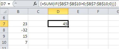
The examination of each cell in the range $B$7: $B$10 (or greater than zero) in the memory array is formed {TRUE, FALSE, TRUE, TRUE}. Then another table is created. If the first array element is TRUE, the second table shows the value of that cell. If the value is “false”, the second element in the array may be zero. After this operation, the first array is removed from the computer’s memory and, ultimately, the IF function returns the array {23, 0, 15, 7}. This array is then passed as an argument to the SUM function, which, in accordance with its intended purpose, returns the sum of all elements in the array. In our example 45. Finally, see what happens even if we ask Excel treats the above formula in an array of notes.

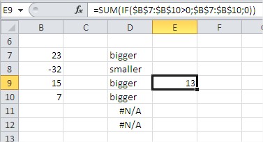
None of the above tables will not be in such a case created. Only one cell range to be tested (cell line, in which the function). In our case 15> 0, so the first argument of the IF function receives the value TRUE. Then passed to the SUM function is the entire range B7: B10, and consequently the function returns a value of 13 (23-32 15 +7). If the cell instead of 15 was the number less than zero IF function as an argument to be given the value FALSE, and consequently to the SUM function would be given only the value zero. Our SUM would return the result as zero.

Example 2 – array transpose function

TRANSPOSE function is a simple example of Table Functions that Excel offers quite a lot. Because they are rarely used in business and are useful primarily for advanced math and statistics, the other array functions will not be discussed in this course. Select range F3: H3, in which you want the resulting array, the introduction of array functions always start by pressing the F2 key.

You type an array function =TRANSPOSE (C3: C5) following array functions always:

You end typing pressing Ctrl + Shift + Enter.

As a result of these activities in cells F3: H3, we feature an array stored in curly braces {}. Although the function ‘looks as if it was placed in three cells, this is one feature, and make changes in any of the cell causes changes in all cells.

Changes to the beginning of pressing F2, and after the introduction of ‘exit’ from an array function by pressing Ctrl + Shift + Enter.

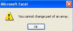
In case of an array of arrays change is not possible, such as in the example above, you can not add a column between the ‘F’ and ‘G’. There will also be possible to introduce any changes other than by pressing F2 to start and end with Ctrl + Shift + Enter. For all such attempts will be displayed:

The function simply delete the array by selecting the entire range in which it is located and press ‘Del’.

I was a little on this. It was to be only about identifying the function of array, and ended up on the description of how they work. It seems to me that the proper “diagnosis” is entirely dependent on an understanding of how the arrays in formulas. When you realize you could say that a particular formula should be entered as an array formula.

Of course, introduced as a non-arrayed can return some output (which you may have to just convince yourself). But if you understand the mechanism, you will see that this result is poor and to work properly it is necessary, however, Ctrl + Shift + Enter. Like anything, understanding and use of the array formulas takes practice. But it is worth spending some time to understand everything. Tables in the formulas allow for the solution of many problems that at first glance appear to be unsolvable.