Adding Graphics

MS Excel or Microsoft Excel is a great tool for organizing data in a spreadsheet. When visualizing data in a spreadsheet, Excel has several options. It allows users to add or insert different graphic objects, such as images, shapes, clip-arts, text-boxes, etc. By adding different graphics, we improve the visual appearance and increase the overall effectiveness of our Excel worksheet.

In this article, we are discussing various graphics objects present in Excel along with step-by-step tutorials on how we can insert any desired graphic object in our Excel worksheet.

How to add/ insert graphics in Excel?

Since Excel has a wide variety of graphic objects, we can add/ insert the desired type of graphic accordingly. However, the process of inserting different graphic objects is slightly different for each graphic. Besides, almost all the graphic objects are present under the Insert tab.

Let us now understand some of the most common graphic objects in Excel, including procedures for adding them to our sheets:

• Adding Picture Graphics
• Adding ClipArt Graphics
• Adding Shapes Graphics
• Adding Chart Graphics
• Adding SmartArt Graphics
• Adding WordArt Graphics
• Adding Textbox Graphics

Adding Picture Graphics

Picture graphics (commonly called images or photos) are one of the most common types of graphics used to enhance the visualization of an Excel sheet. Adding pictures to an Excel sheet is a fairly easy task. Additionally, we can choose the desired images from various sources. The two most common sources include local storage and the Web.

Adding Picture Graphics from the Local Storage

It often happens that we may need to add pictures from local storage, which we have saved earlier. For this, we need to do the following steps:

• First, we need to open an Excel sheet to which we want to add a picture(s).
  
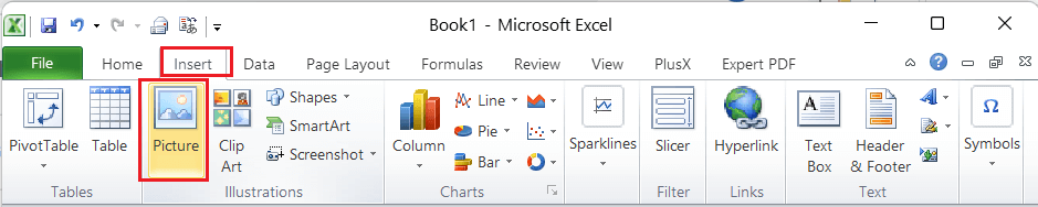
• Next, we need to navigate the Insert tab and click the ‘Picture‘ tool from the ‘Illustrations‘ group.
  
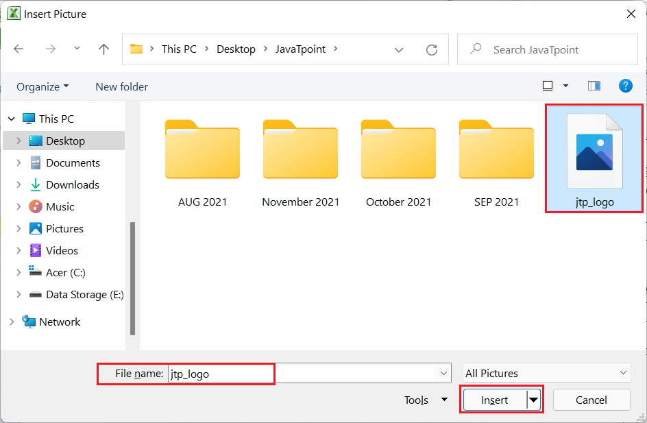
• After clicking the ‘Picture’ tool, we need to browse pictures using the ‘Insert Picture dialogue box’. We can filter the specific picture format using the drop-down list next to ‘All Pictures’.
  After locating the desired picture, we must double-click on it using the mouse to insert it into our current worksheet. Alternately, we can click the ‘Insert‘ button to do the same task.
  
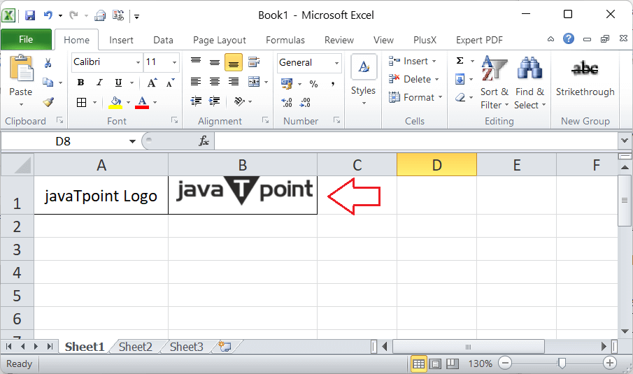
  Once the picture is inserted into our worksheet, we can adjust its size by dragging the corner edges. Furthermore, we can adjust the height and width of the Excel cells to fit the inserted picture in them.
  

Adding Picture Graphics from the Web

There are multiple methods to insert a picture from the web into our Excel worksheet. The most common methods are as follows:

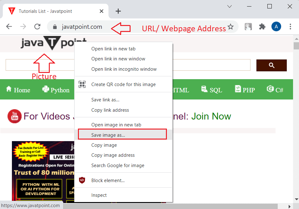
• Saving and Inserting: We need to first navigate to the webpage from which we want to take a picture to add to our Excel worksheet. We must right-click on the specific picture on the webpage and select the ‘Save image as‘ option from the list.
  
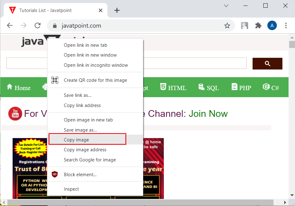
  After that, we need to save the picture to a desired local folder. Once the image is saved into our local storage, we can follow the method discussed above in this article.
• Copy-Pasting: If we don’t want to save specific images to our local storage, we can directly copy them and add them to our excel sheet. Like the previous method, we need first to navigate the web page and press the right-click on the particular picture. Next, we need to select the option ‘Copy Image‘ from the list.
  
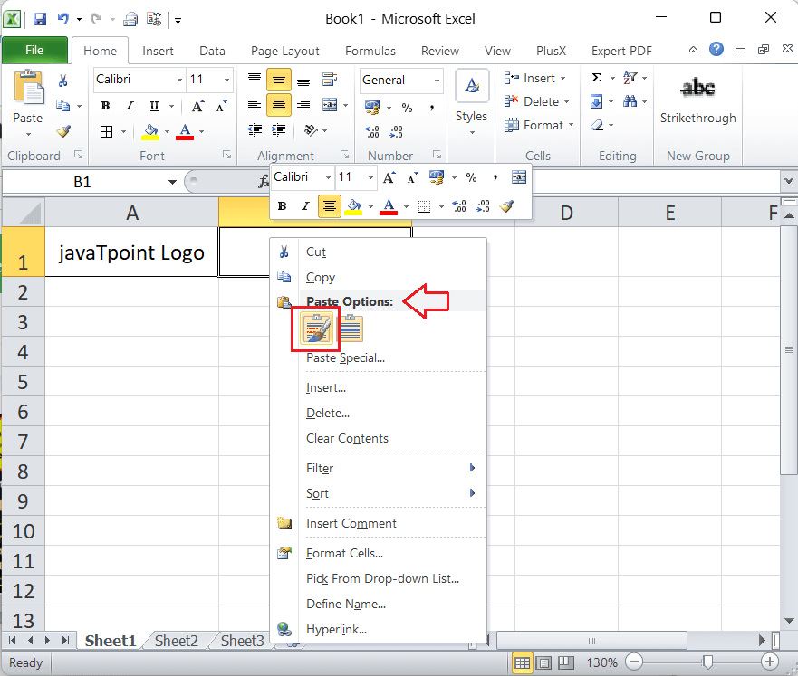
  After the desired picture is copied, we must go back to our Excel sheet and right-click again. Lastly, we must click the ‘Paste‘ option. Furthermore, we can adjust the size of the picture accordingly.
  

Adding ClipArt Graphics

Clip Art is another popular graphic object designed using various pictures in different categories like animals, people, schools, etc. This type of graphic can easily be imported into any other document, such as Word, Excel, PowerPoint slides, etc.

We can perform the following steps to insert clip art into our Excel worksheet:

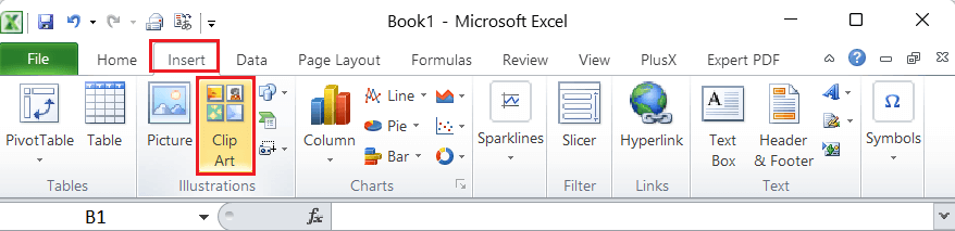
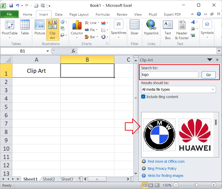
• First, we need to go to the Insert tab and click the ‘Clip Art‘ option.
  
• We need to type the relevant keyword into the Search Box and press the Enter key in the next window. This will display various clip-arts according to our searched keyword.
  
• Lastly, we must double-click on the desired clip art, and it will be instantly inserted into our worksheet.
  

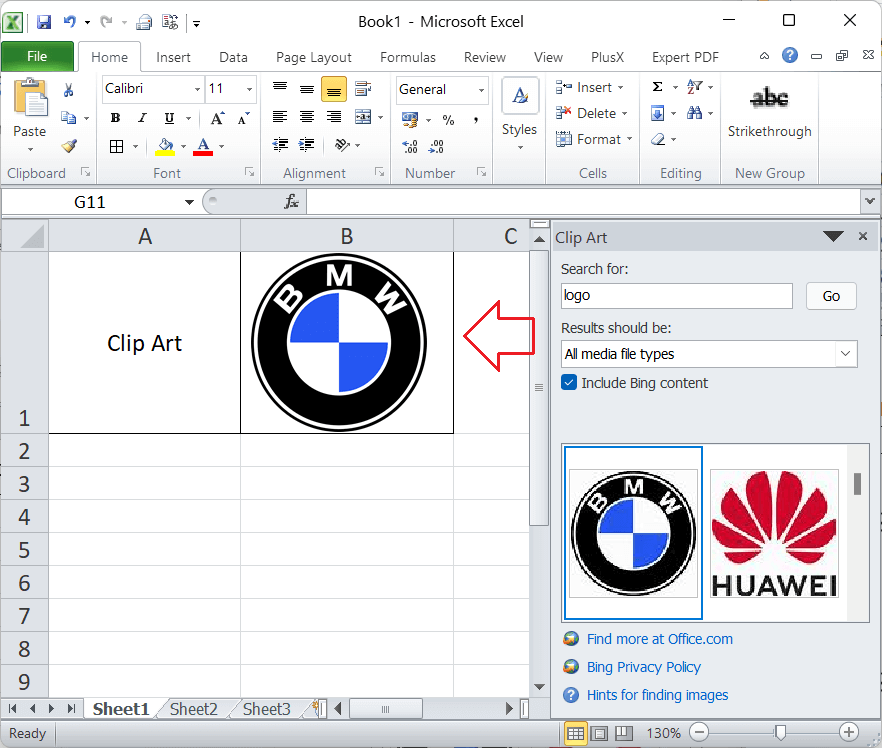
After the clip-art is inserted into our worksheet, we can adjust the height and width by dragging the corner edges. Alternately, we can select the specific clip art and then manage preferences from the Format tab.

Adding Shapes Graphics

The shape plays a crucial role in visualizing the worksheet interface, and it can help illustrate the organized data in different styles. It is easy to add shapes into our Excel sheet and combine shapes to form any specific logo or design.

We can insert the desired shape by performing the below steps:

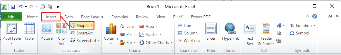
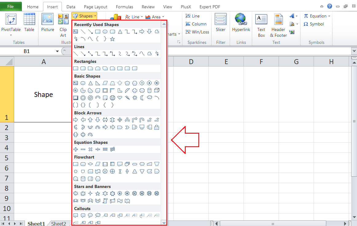
• First, we need to navigate the Insert tab and click the drop-down icon associated with the text ‘Shapes‘. This will display various built-in shapes present in Excel.
  
• We can click on the desired shape in the next window and draw it using the mouse within the active sheet.
  

In this way, we can add multiple desired shapes into our Excel sheet. If we create any specific design by using various shapes, we can group them as one shape. For this, we must select each of the added shapes by holding the Ctrl key and then click the option ‘Group‘ from the Arrange section on the ribbon.

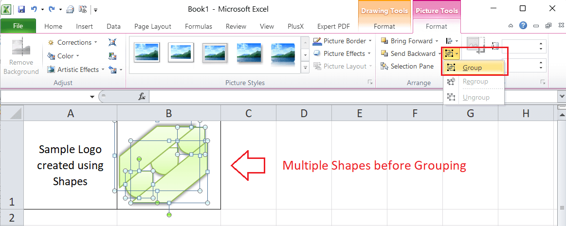
When combining various shapes as a single object, we can easily move and resize them as one entity. We don’t need to move/ resize each shape one by one. For example, creating a logo by adding and grouping multiple shapes within the sheet.

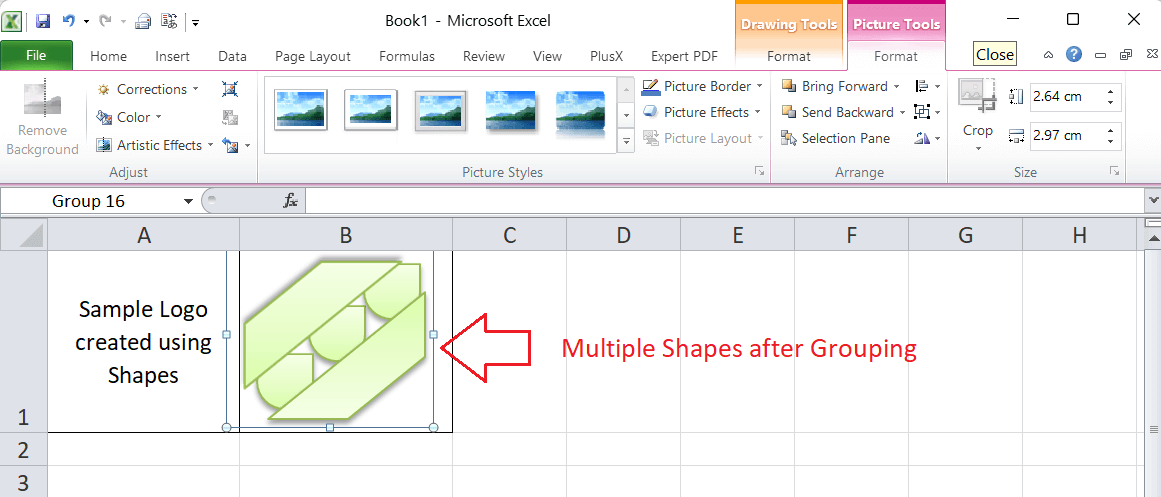
In the above image, all the shapes have been combined and are acting as a single entity. Similarly, we can add as many shapes as we need to create a specific desired design.

Adding Chart Graphics

Excel has various built-in charts that help visualize the data within the spreadsheets. Charts can summarize the important data with results in a small area, and they can save time to make any conclusion based on the supplied data. However, we must have a basic understanding of using Excel charts to choose the appropriate chart as per our data sets. Some essential charts in Excel are the Line chart, Bar chart, Column chart, Pie chart, Doughnut chart, etc.

The following are some common steps of inserting the desired chart in an Excel sheet:

• First, we must enter the data within the Excel sheet.
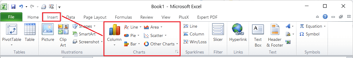
• Next, we must select the appropriate range of entered data sets and go to the Insert We need to select the desired chart from the group named ‘Charts‘.
  

Once the selected chart is inserted into our worksheet, we can customize the chart elements accordingly. Besides, we can also change the chart types whenever we may need them.

Let us create a simple chart (Line Chart) to understand better the process of adding chart graphics into an Excel sheet:

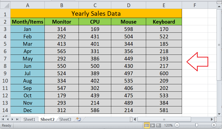
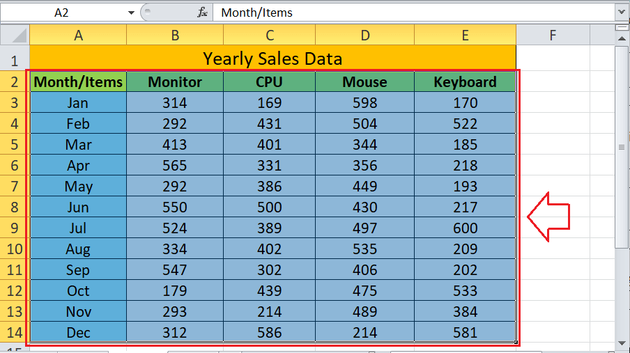
Consider the following Excel sheet with some sales data as an example data set.

Now, we will create a simple line chart that will display the sheet data through graphic representation. We must execute the following steps:

• First, we need to select the effective range of data. In our case, we select the range A2:E14, as shown below:
  
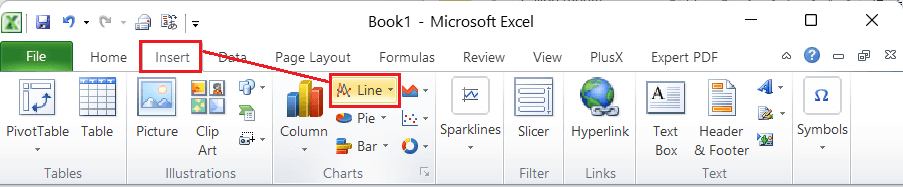
• Next, we need to go to the Insert tab and click the drop-down icon associated with ‘Line‘ in the ‘Charts‘ group.
  
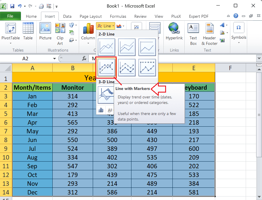
• After that, we need to select the tile named ‘Line with Markers‘.
  
  This will immediately add the corresponding chart for the selected range of data.
  

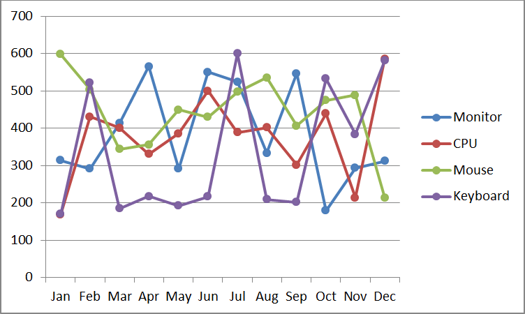
In the above chart, we can understand the estimated sales data for each month for each item. In this way, we can add chart graphics to our Excel worksheet.

Adding SmartArt Graphics

The SmartArt graphics allow users to quickly add a variety of presentation designs, such as flow charts, block-lists, hierarchy diagrams, etc. We can select the desired SmartArt from different categories, including the list, process, cycle, hierarchy, etc.

We can add the desired SmartArt graphic by performing the steps discussed below:

• First, we need to launch or open an Excel sheet to which we want to add Smart graphics.
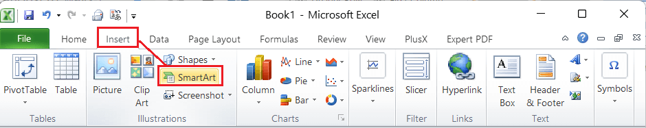
• Next, we need to go to the Insert tab and click the ‘SmartArt‘ option, as shown below:
  
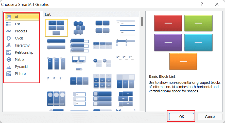
• In the next window, we can choose the desired SmartArt graphic amongst different categories.
  
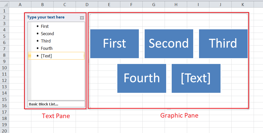
  Once the selected SmartArt graphic has been inserted within the Excel sheet, we will get the two panes. The first pane is where we can enter text contents to reflect them into our graphical representation, and the text pane is located on the left side. On the other hand, another pane (right-side pane) displays the exact appearance of the inserted SmartArt graphic.
  

Adding WordArt Graphics

Like MS Word, Excel also allows users to add WordArt graphics within the active sheet. Using this type of graphics, we can enter stylized text or Word Art objects into the worksheet.

We can add the desired WordArt graphic by executing the following steps:

• First, we need to open an Excel sheet to insert a WordArt graphic and navigate the Insert tab on the ribbon.
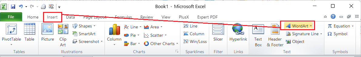
• Next, we must click the ‘WordArt‘ option, as shown below:
  
  In the next window, we need to click the desired WordArt object.
  
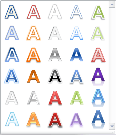
  This will immediately insert a selected WordArt into our sheet where we can enter the desired text using the keyboard.
  
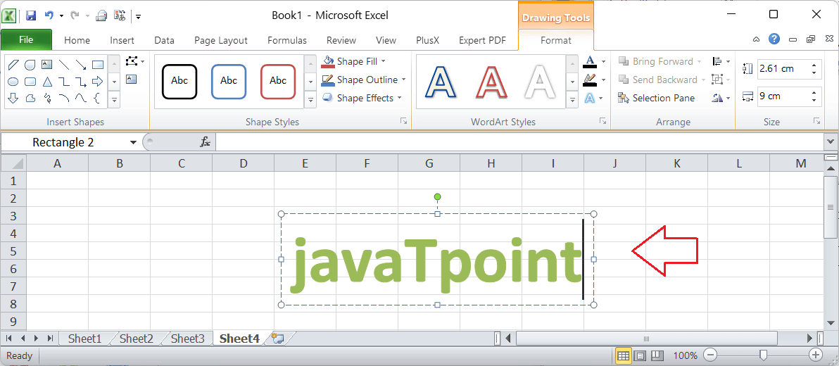
  After the desired WordArt object has been added, we can adjust shadows, reflections, color glow, and many other preferences to make it more attractive.

Adding Textbox Graphics

We can add text boxes with various styles to our worksheet. The text boxes mainly help visualize the text content and make it look attractive and eye-catching. Therefore, we can enter some essential information into such boxes and position them anywhere within the Excel sheet, irrespective of Excel grids.

To add a text box into our Excel worksheet, we need to perform the following steps:

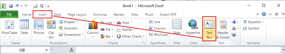
• First, we need to go to the Insert tab and then select the ‘Text Box‘ option, as shown below:
  
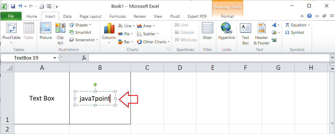
• As soon as we click on the ‘Text Box’, the corresponding tool is activated. After that, we need to click on the excel sheet, and Excel will add a default text box with empty text into our current sheet.
  
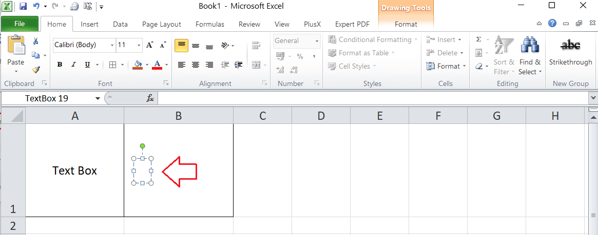
• Once the text box is inserted, we can click inside the box and type the content we want to insert. Despite this, we can move the text box by dragging it using the mouse. The text content inside the text box will also be moved accordingly.
  
  It is a good practice to try different styles to make the text box more attractive. Although we can manage the different styles manually, we also have some built-in styling options.
  

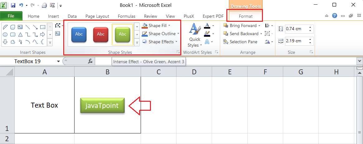
The text box graphic is more beneficial than the normal text. This is because we can adjust the formatting of the box, box color, text color, border color, etc.

Important Points to Remember

• Almost all graphics can be added from the Insert tab on the Excel ribbon.
• It is best to adjust the height, width, style, and other formattings of the included graphics to match the current theme of our worksheet.
• We can use the Alt key while dragging the picture’s edges with the mouse to adjust the picture size to the extreme corners of Excel cells.
• To select multiple graphics in an Excel sheet, we can press and hold the Ctrl key while selecting them using the mouse.