Excel round off formula
If you do not want to store decimal points in your Excel cell, you can round off the value to the nearest unit. Excel offers in-built functions to achieve this goal. It removes the unnecessary decimal points from the value and the value changes from floating-point number to an integer.
A value can be round off in various ways that we will show you in this chapter. Excel offers in-built functions to achieve this goal. Apply them on your floating-point data and round off the value. Additionally, you can also round a number to the nearest major units, such as ones, tens, hundreds, or thousands using these functions. It means that – the user can also customize the nearest unit to round off.
In this chapter, we are going to use Excel formulas in different ways to round off the values.
Rounding functions in Excel
As we already told you that, Excel offers several in-built functions to round off the decimal point values, which are –
| Function | Description |
|---|---|
| ROUND | It is used to round the value normally. |
| MROUND | It rounds the value to the nearest multiple. |
| ROUNDDOWN | It rounds down to the nearest place specified in this function. |
| FLOOR | It rounds down the value to the nearest specified multiple. |
| ROUNDUP | It rounds up to the nearest place specified in this function. |
| CEILING | It rounds up the value to the nearest specified multiple. |
| INT | It rounds off the value to the nearest integer number. Means that – this function rounds off and returns only an integer number. |
| TRUNC | This function only TRUNC the decimal point from the number and returns the value. |
Each function is a bit different in working from each other and provides different results. However, they all are used for rounding off the decimal point from number in Excel. Use them according to your need. We will show you examples for every function.
How to use these formulas in an Excel worksheet?
There are two ways of using the following formulas in the Excel worksheet. Either you can use them from the FORMULA interface or by writing the formula in the formula bar.
Formula Interface
On the Excel dashboard, go to Formulas tab > Math & Triangle > list of formulas.
Whenever a user selects any formula from this Math & Triangle dropdown list, its respective interface opens here, as showing for the ROUND formula.
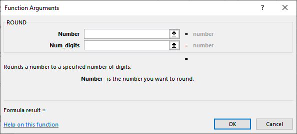
If you are not good at remembering formulas, this method is good for you.
Formula bar
Besides the Formula interface, you can also apply and execute any formula directly on your Excel worksheet by typing them into the Formula bar. This is helpful when you know the formula.
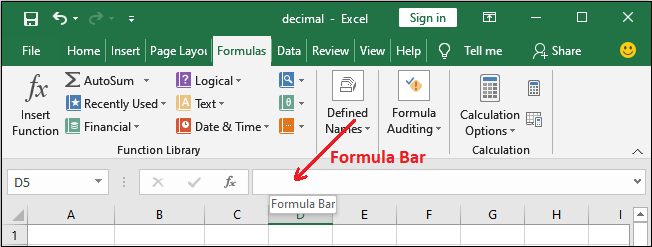
It is a bit faster than the above one, if you remember with Excel formulas.
ROUND()
The ROUND() function in Excel is used to round off the values with decimal points normally that we do in our daily maths. It returns the value after rounding off to its nearest value.
It keeps the last digit accordingly after rounds off.
Syntax
The first parameter is number parameter that you want to round. Another is num_digits that is the number of digits to be round in number value.
Example
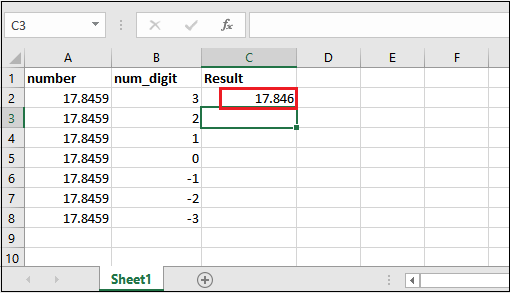
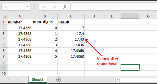
We have values with decimal points to which we will round off using the ROUND() function for different values in the num_digits. Now, let’s see how the ROUND() function works on these values.
Step 1: Type the ROUND() formula in the Formula Bar for the 1st row data.
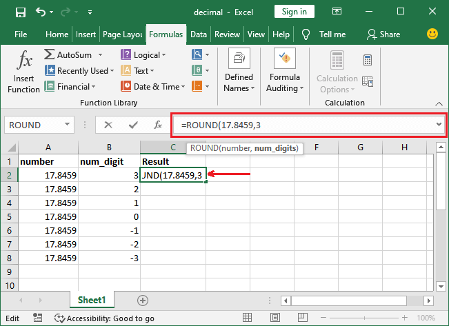
Step 2: Press the Enter key to get the result after round off the value.
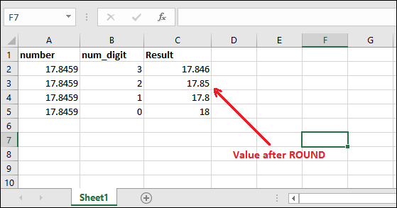
Step 3: Apply the ROUND formula on all the given values and see the result for different values in the num_digit parameter.
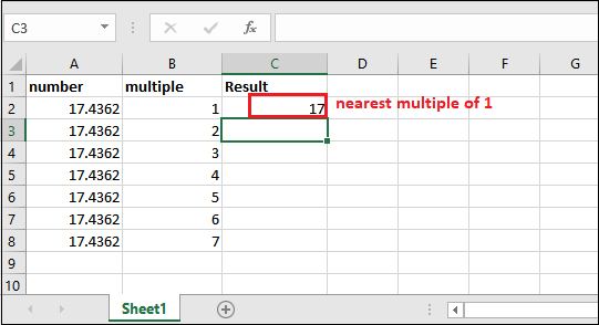
MROUND()
The MROUND() function rounds the values to the nearest multiple. It returns the value after rounding off to its multiple. For example, for a number 19.8462, the nearest multiple of 7 is 21. The given number lies between 14 and 21, which are multiple of 7. Here, you can see the 21 is nearest to 19.8462. So, the result is 21.
Syntax
Here, number is a parameter that you want to round off and multiple is another parameter that contains a digit to round off the number to its nearest multiple.
Example
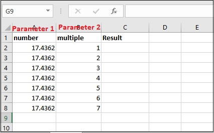
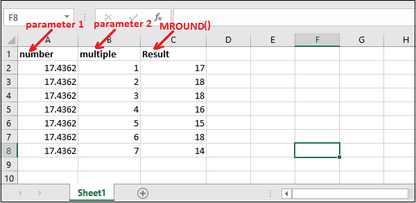
To understand the working of this formula, we have an Excel dataset of floating-point values. We will round off the values to the nearest multiple using the MROUND() function for different multiple. Now, let’s see how MROUND() function works on these values.
Step 1: Type the MROUND() formula in the Formula Bar for the 1st row data.
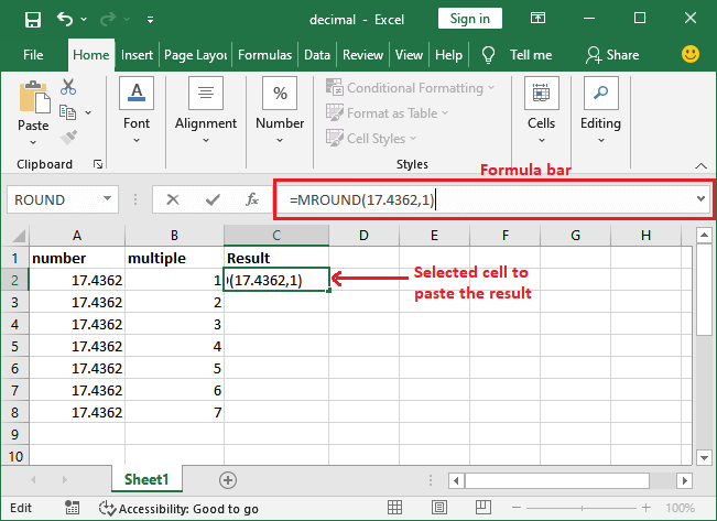
Step 2: Press the Enter key to get the result after round off the value.
Step 3: Apply the MROUND function on all the given values and see the result for different values of multiple parameter.
ROUNDDOWN()
The ROUNDDOWN() function in Excel, rounds down the specified value to its nearest integer. It returns the value after rounding off. This function is much similar to the ROUND() function.
It just removes the extra digits from the value after the decimal point and only keeps the number of digits specified in the function.
Syntax
The first parameter is number parameter that contains a floating-point you want to rounded down. Another is num_digits that is the number of digits to be round in number value.
Example
Let’s take an example and understand how it is different from the ROUND() function.
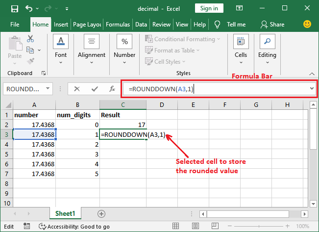
Here, we have the following Excel dataset containing some real numbers on which we will apply ROUNDDOWN() function.
Step 1: Select a cell to paste the rounded result and go to the formula bar to execute the ROUNDDOWN() formula.
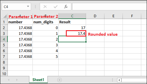
Step 2: Press the Enter key to get the rounded value and see the result.
Now, we will apply the same function on all other values present in this Excel worksheet.
Step 3: See the result after rounding down all given values with different values of the num_digits parameter.
FLOOR()
The FLOOR() function in Excel is used to rounds a number down to the nearest multiple of the specified significant. It returns the value after rounding off to the nearest value of the multiple.
Syntax
The number parameter accepts the floating-point value you want to round off. The second parameter is significant that contains a digit to round off the number to its nearest multiple.
Note: The FLOOR() function is deprecated now and FLOOR.MATH() comes as its option that contains one more parameter named mode, which is optional.
Example
Let’s take an example and understand how this function actually works.
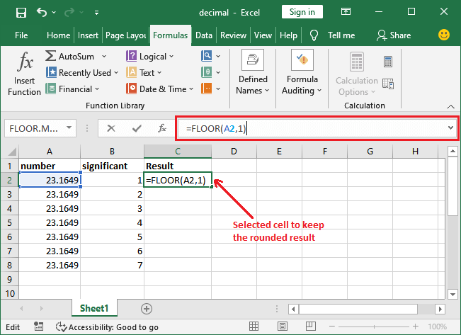
Here, we have the following Excel dataset containing the same real number in number field and different in the significant field on which we will apply the FLOOR() function.

Step 1: Select a cell to paste the rounded result and go to the formula bar to execute the FLOOR() formula.
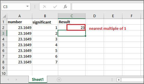
Step 2: Press the Enter key to get the rounded value and see the result.
Now, we will apply the same function on all other values present in this Excel worksheet.
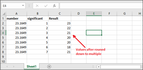
Step 3: See the result after rounding down the given values with different values of the num_digits parameter.
ROUNDUP()
ROUNDUP() function is opposite to the ROUNDDOWN() function. As the name implies, the ROUNDUP() function in Excel, rounds up the number to the nearest integer. It returns the value after rounding off. This function is much similar to the ROUND() function.
It just removes the extra digits from the value after the decimal point and only keeps the number of digits specified in the function.
Syntax
The first parameter is number parameter that contains a floating-point number you want to round up. Another is num_digits that is the number of digits to be round in number value.
Example
Let’s take an example and understand how it provides just opposite results to ROUNDDOWN() function.
We will take the same dataset used for ROUNDDOWN() function, but this time, we will apply the ROUNDUP() function on it.
Step 1: Select a cell to paste the rounded result and go to the formula bar to execute the ROUNDUP() formula.
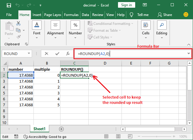
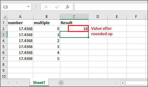
Step 2: Press the Enter key to get the rounded value and see the result.
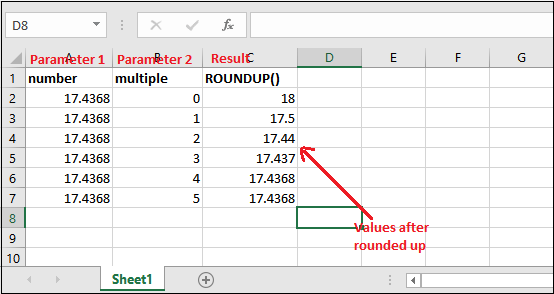
Now, we will apply the same function on all other values present in this Excel worksheet.
Step 3: See the result after rounding down all values for different multiple parameter values.
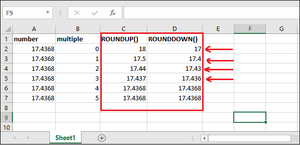
Note the result for both ROUNDDOWN and ROUNDUP for the same dataset to see its difference in resultant data.
CEILING()
The CEILING() function is opposite to the FLOOR() function. This function is used to rounds a number up to the nearest multiple of the specified significant. It returns the value after rounding off to the nearest value of the multiple.
Syntax
The number parameter will contain a floating-point value you want to round off. The second parameter is significant that accepts a digit to round up the number to its nearest multiple.
Note: Just like the FLOOR() function, CEILING() function is deprecated now and CEILING.MATH() comes as its option that contains one more parameter named mode, which is optional.
Example
Let’s take an example and understand how it different than FLOOR().
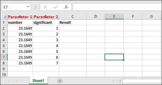
Here, we have the following Excel dataset containing the same real number in number field and different in the significant field on which we will apply the CEILING() function.
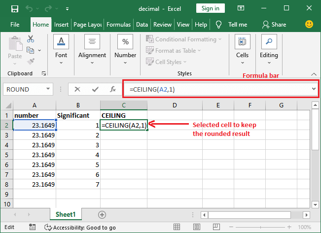
Step 1: Select a cell to paste the rounded result and go to the formula bar to execute the CEILING() formula.
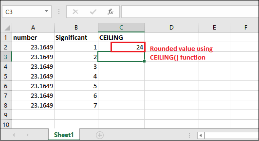
Step 2: Press the Enter key to get the rounded value and see the result.
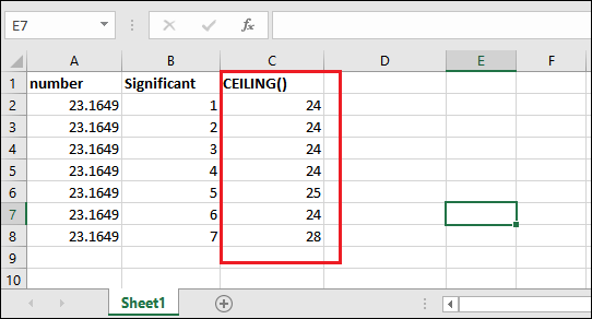
Now, we will apply the same function on all other values present in this Excel worksheet.
Step 3: See the result after rounding up the given values with the multiple of different significant parameter value.
Note the result for both CEILING() and FLOOR() for the same dataset to see its difference in result value.
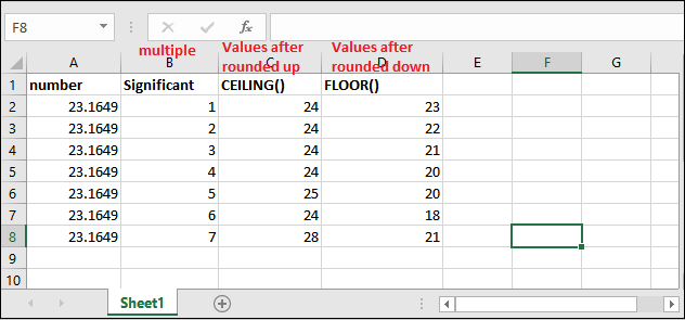
By applying both CEILING() and FLOOR() functions with the same parameter values, it is easy for the users to understand the working and difference of both functions.
INT()
The INT() function is similar to all the other methods discussed above with a minor difference. In Excel, this function is used to round off the value to the nearest integer number. Means that – this function rounds off and returns only an integer number. It will be the simplest method to round off the real number for users.
Now, we will take an example to understand the working of this function. Before this, see the syntax of INT() function, as following:
Syntax
The INT() function does not require any extra parameter. It takes only one parameter named number that accepts a floating-point number you want to round off.
Example
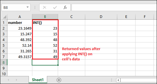
Now, let’s see an example with data in an Excel table. For this, we have the following data.
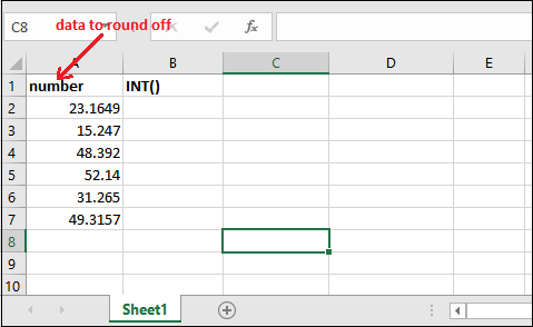
Step 1: Select a cell to keep the respective cell result after rounded off and go to the formula bar to execute the INT() formula. For the A2 cell,
=INT(A2)
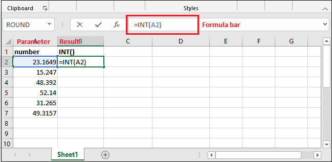
Step 2: Press the Enter key on your keyboard and get the resultant value.
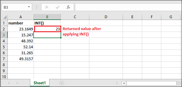
Step 3: Similarly, execute the same function for all other cell’s data by just changing the cell number. See the result after applying the INT() on all data.
The last formula to round off the real numbers in Excel is – TRUNC().
TRUNC()
The TRUNC() function is the last function to be discussed in this chapter that is used to round off the real numbers in Excel. Same as the other round off function, it also enables the Excel users to round off the Excel data.
Syntax
The first parameter is number parameter that accepts a floating-point number you want to rounded down. Another is num_digits that is the number of digits to be round in number value
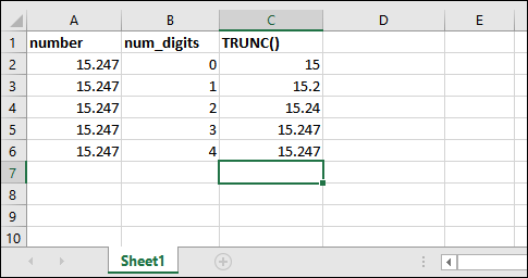
Example
Now, let’s see an example with data in an Excel table.
Step 1: Select a cell to keep the respective cell result after rounded off and go to the formula bar to execute the INT() formula. For the A2 cell,
=INT(A2)
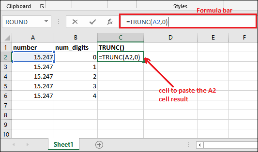
Step 2: Press the Enter key on your keyboard and get the resultant value.
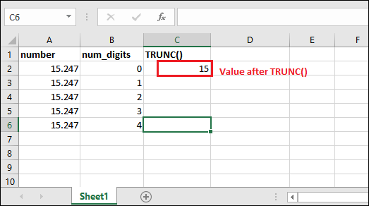
Step 3: Apply the same formula on all other cell’s data and see the result.