How to calculate percentage in Excel

MS Excel, short for Microsoft Excel, is powerful spreadsheet software that enables users to record numbers in various forms in cells across multiple worksheets. It also gives the flexibility to perform various calculations or operations or recorded data or numbers using specific functions and formulas. While working on Excel, there may be times we need to find or calculate percentages. Although it seems quite difficult to calculate percentages in maths, it is comparatively very easy in Excel.

This article discusses various scenarios and related step-by-step tutorials on calculating percentages while working on Excel. The article also includes examples of different scenarios when we might need to calculate percentiles. Before we discuss how to calculate percentage in excel, let us first discuss the basic mathematical fundamentals of percentage.

Basics to Calculate Percentage

In mathematics, the percentage is defined as an operation that involves multiplying the fraction by 100. In other words, a percentage is a fraction of 100, which is calculated by dividing the numerator value by the denominator values and further multiplying its result by a hundred. The term ‘percent (per cent)’ belongs to Latin and is extracted from ‘per centum’, which means ‘by the hundred’.

The basic mathematical formula of percentage is defined as:

For example, if a student gets 475 marks/numbers in six different subjects where each subject has a maximum of 100 marks to score, then a student scores 475 out of 600. In that case, if we need to calculate percentage mathematically, we have to divide the scored marks (475) by the total number of maximum marks (600) and multiply the fraction result by 100, i.e.:

(475/600)*100 = 79.16

Thus, the student scored 79.16%.

Excel Percentage Formula

Calculating multiple percentages mathematically would be quite difficult and prone to errors. However, we can easily calculate hundreds of percentiles in Excel without making errors. Percentage calculator is a useful function that helps us calculate percentages in excel. It is not technically a function but a set of mathematical operations.

The basic formula to calculate percentage in Excel is defined as:

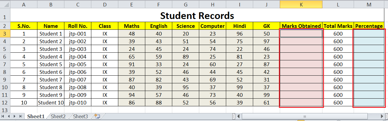
Let us now consider the example where we have to calculate the percentage of marks of several students instead of just one student. Excel will help us calculate their subjects’ total and calculate the percentage automatically. Consider the following example sheet as an example:

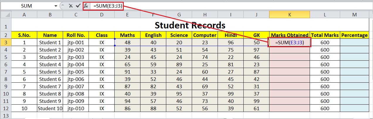
In the above image, we can apply the SUM function to calculate each student’s total number of marks. Thus, we apply the SUM function in cell K3 by supplying all subjects’ marks, as shown in the following image:

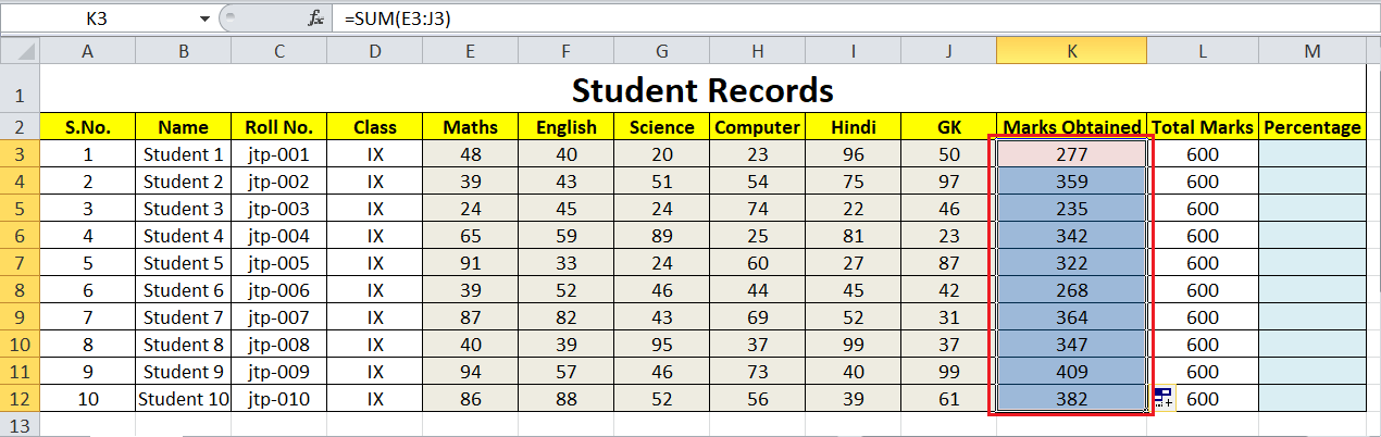
Now, we drag the formula to the bottom of the column to calculate the total number of marks for each student separately.

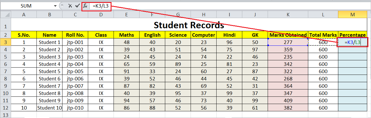
After calculating the total obtained marks, we must calculate the percentage. Thus, we apply the percentage formula in cell M3 for the first student like this:

Percentage = Marks Obtained / Total Marks

i.e.,

Percentage = cell K3/ cell L3

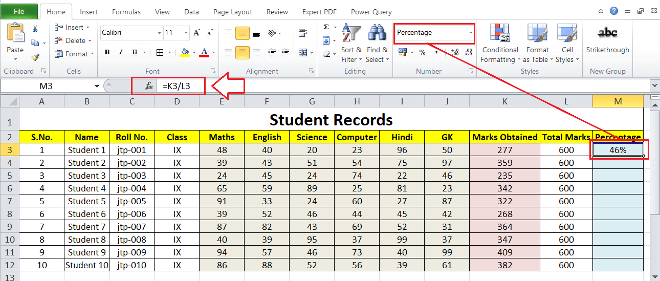
After applying the above formula, we must change the cell format to the percentage by clicking the percentage sign in the Number section under the Home tab. Alternately, we can press the keyboard shortcut ‘Ctrl + Shift + %‘ to immediately convert the output to a percentage. That’s why we don’t multiply the fraction result by 100 when calculating the percentage in Excel.

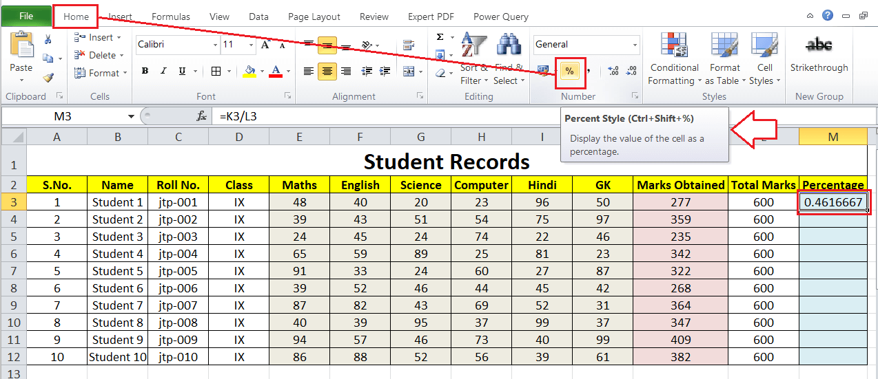
This way, we calculate the percentage of marks for the first student.

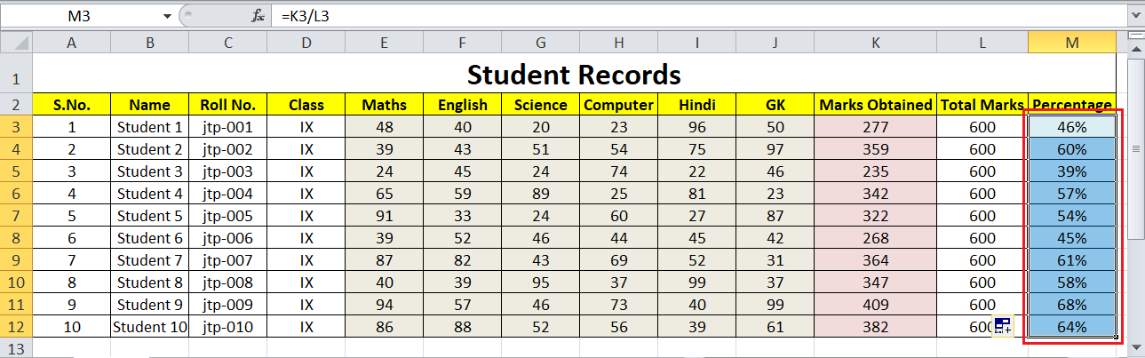
Lastly, we must drag the formula from cell M3 to the bottom of the column to calculate the percentage of marks for other students. The final table will look like this:

This is how we usually calculate percentages in general. However, it is only a normal case. We may have various specific cases to find percentages.

Calculating Percentage for Specific Cases in Excel

Excel offers multiple ways to calculate the percentage of recorded data. For instance, we may need to use Excel to calculate the percentage of correct answers out of total submitted answers, prices after discounts based on certain percentages, percent changes between two different values, or after increase or decrease. There may be several cases based on the requirements. However, calculating percentages using Excel is quite easy in all such cases.

The following are some of the most common cases with relevant examples that will help us calculate percentage in Excel on different data sets whenever required:

Calculating a Percentage as a Proportion

The previous example under the Excel percentage formula is a specific case of calculating percentage as a proportion or calculating the percentage of a total. Whenever we need to calculate the size of a particular sample as a percentage of the entire set, we can divide the sample portion by the size of the entire set.

For instance, if we have got 90 marks out of 120 in any subject, we can calculate our percentage score of a particular subject by dividing 90 by 120. We must type the formula in an Excel cell like this:

=90/120

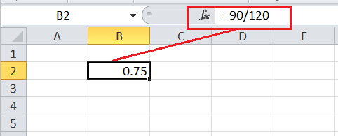
In the above example sheet, the result is given as 0.75. Changing the cell format to percentage will change to 75%, meaning we scored 75% in that corresponding subject.

Let us now discuss some other examples of this particular case so that we can better calculate the percent of the total on different data sets or proportions using Excel:

Example 1: Calculating percentage as a proportion when a certain cell has a total at the end of the table

One of the common cases is when we have data in multiple cells of a column, and the total is given at the end of the column in the respective table. We can apply the percentage formula similar to the previous example in such cases. However, since the total is listed at the end of the table in a column, we must ensure to use an absolute reference (with $). Using the absolute reference, we fix the cell reference with a total so that it does not change even if we copy the formula to other cells in the sheet.

Suppose we have values in column B from B2 to B9, and their total is given in cell B10. We can apply the following percentage formula in cell C2 to calculate the percentages as a proportion (percentage of total) for the product listed in cell A2:

=B2/$B$10

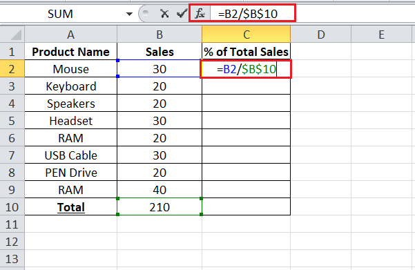
In the above example sheet, we can see a relative cell reference used for cell B2. Therefore, if we drag the formula from B2 to B9, the cell references on the numerator will accordingly change to B3, B4, B5, and so on. However, the absolute cell reference ($B$10) remains the same.

The following image displays the percentages of the total as proportions where the respective column (column C) is formatted as the percentage with 2 decimal places:

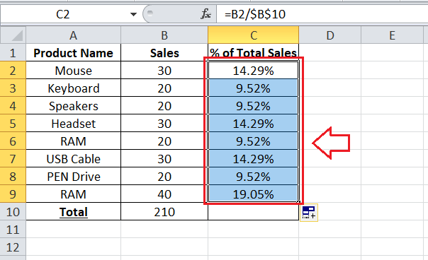
The above image shows the proportion of each product as the percentage of total sales.

Note: To use an absolute reference in Excel, we have to manually enter the dollar sign ($) or press the F4 function key after placing the cursor over the corresponding cell reference in the formula bar.

Example 2: Calculating percentage as a proportion when parts of total are present in multiple cells/rows

In addition to the previous example, suppose that the sales of any specific product are divided or listed in multiple rows, and we need to calculate the percentage of that product. In such a case, we can take advantage of the SUMIF function. First, we sum up all the respective values of a product and then divide the added result by the total. We can apply the SUMIF function in Excel like this:

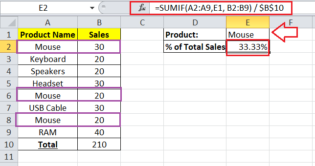
Like the previous example, if we enter product names in column A, their sales in column B, total in cell B10. However, the product for which we want to calculate the percentage is written in cell E1. Therefore, we calculate the percentage proportion of certain products in cell E2 like this:

=SUMIF(A2:A9 ,E1, B2:B9) / $B$10

The above formula works universally, meaning that we can enter the name of other products of our range, and the respective percentage proportion will be calculated automatically.

Apart from this, we can also enter the desired product name directly within the formula like this:

=SUMIF(A2:A9, “Mouse”, B2:B9) / $B$10

The above formula will also give the same result; however, we cannot use it for calculating percentages proportion other products. We have to edit the formula again and change the product name in the formula accordingly.

In addition to this, if we need to calculate the percentage proportion of more than one product, we can add the respective values and combine them using multiple SUMIF functions. For instance, the following formula in our example will calculate the percent of Mouse and Keyboard out of the Total:

=(SUMIF(A2:A9, “Mouse”, B2:B9) + SUMIF(A2:A9, “Keyboard”, B2:B9)) / $B$10

Calculating Percentage Change

Calculating the change (increase or decrease) in percentage is one of the most common tasks, and we mainly prefer Excel to calculate it. Generally, when we need to calculate the percentage change between the two different values, A and B, using Excel, the following formula works well:

However, when using the above formula in Excel, we must be aware of selecting the A and B properly from our data set. Thus, to be more specific, we can define Excel’s percentage change formula like this:

After applying the formula in the real-time example, we must change the cell format to percentage.

For instance, suppose that any soccer team scored 16 goals last year and 20 goals in the current year. In that case, we calculate the percentage change (an increase of % goals) in the current year as compared to last year with the following formula:

=(20-16)/16

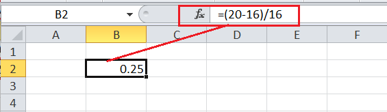
In the above example sheet, the result is given as 0.25. If we change the cell format to percentage, it will change to 25%, meaning a 25% increase in goals from the last year. Now, let us discuss this concept with a real-life example in Excel:

Example 1: Calculating percentage change between columns

Suppose we have some items with their last month’s prices in column B. However, the prices have changed in the current month and are listed in column C. We need to calculate the percent change (increase or decrease whichever applies) in column D. In that case, we must apply the percent change formula in Excel’s cell D2 like this:

=(C2-B2)/B2

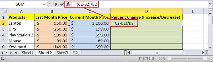
The formula returns the decimal value. We must change the cell format to the percentage by clicking the percentage sign (Ctrl + Shift + %) on the ribbon, which will convert decimals into a percentage.

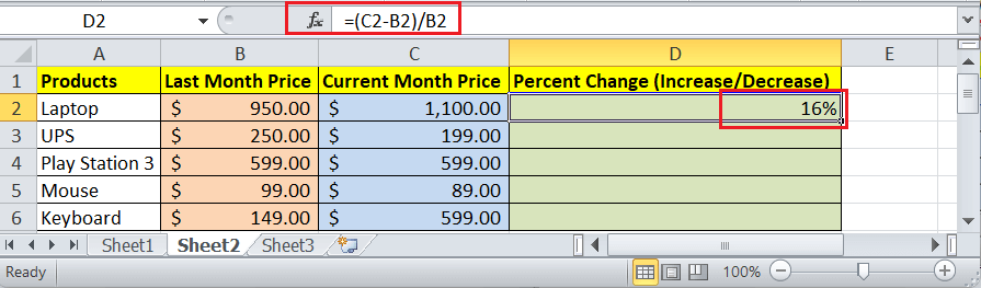
The above formula calculates the percent change for a laptop in the current month (column C) compared to the previous month (column B). If we drag the formula from D2 to other cells of the respective column, we will get the percentage change (increase/decrease) for other products.

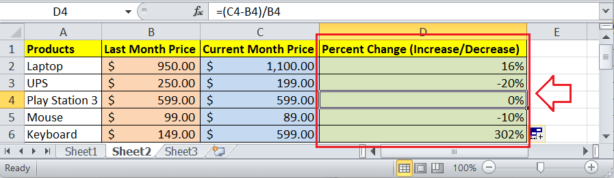
In the above example sheet, we notice positive and negative values in column D. The positive percentages represent the percentage increase (price increase), and the negative percentages represent the percentage decrease (price decrease).

Example 2: Calculating percentage change between rows

Suppose we have month-wise sales data of any item in column B while respective months are mentioned in column A. We need to calculate the percent change (increase or decrease in monthly sales compared to the previous month) in column C. In that case, we must apply the percent change formula in Excel’s cell C3 like this:

=(B3-B2)/B2

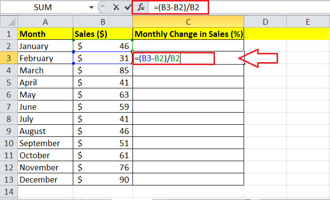
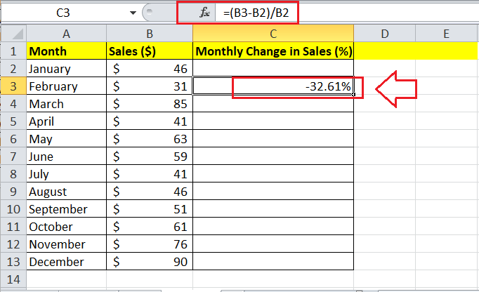
Since January is the initial month, there will be no percent change for this month. That is why we apply the formula in cell C3, not in cell C2. After applying the formula, we must change the cell format to the percentage (Ctrl + Shift + %).

We can drag the formula into other cells of the respective column to calculate the percentage change for other months compared to the previous month’s sales.

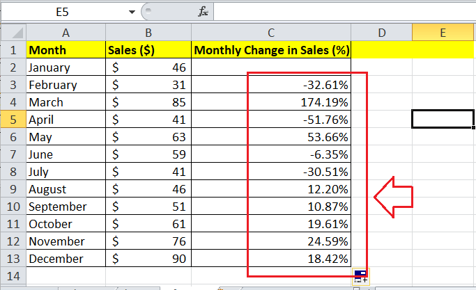
Like the previous example, the positive and negative percentages represent an increase and decrease in sales compared to the previous month.

In addition to this, if we need to calculate percent change compared to any specific month (suppose January) for all other months, we have to fix the cell reference with January sales data using the absolute cell reference feature. In our case, we can fix the January sales data by using absolute reference $B$2.

For example, we can use the following percentage formula in the same example to calculate the percent change (increase/ decrease) for each corresponding month compared to January (B2):

=(B3-$B$2)/ $B$2

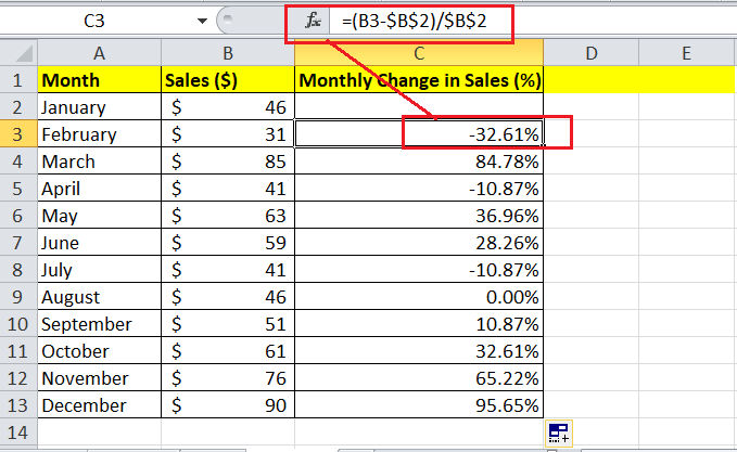
There will not be any effect on the absolute cell reference in the above formula even after dragging the formula from cell C3 to the other cells in the column below. With absolute reference, the cell with the January data ($B$2) is fixed for each result cell (C3, C4, C5,…), while the relative cell reference B3 changes accordingly to B4, B5, B6, and so on.

Calculating a Percentage of a Number

Another common case is calculating the percentage of any specific number in Excel. For instance, we need to calculate the 25% of 50. In such cases, we only need to multiply the percentage value by the given number for which we need to find the percentage, i.e.:

It means, to calculate 25% of 50, we must multiply 25% by 50 in an Excel cell like this:

=25%*50

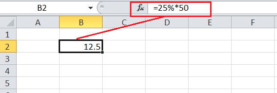
In the above example sheet, the result 12.5 is given, meaning 25% of the number 50. Now, let us discuss this concept with a real-life example in Excel:

Example: Suppose we are buying a laptop which costs $950. However, the seller also asks us to pay an additional 11% VAT on the net price. So, the question would be, how much will we have to pay apart from the net price of the laptop? In the other case, what would be 11% of 950$?

Now, we put all these values in Excel in a manner where the total value of the laptop is recorded in cell A2 and the percent of VAT in cell B2. Let us consider cell C2 as the result cell for calculating the percentage amount. So, we must apply the formula =A2*B2 (Total*Percentage) is the result cell like this:

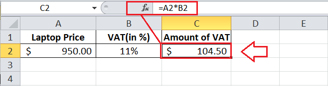
Excel returns 104.50$ as a result, which is the additional VAT amount we need to pay. Therefore, the total money we have to pay equals the laptop net price and the VAT, i.e., 950$ + 104.50$ = 1054.50$.

It is essential to note that when we use a percent sign with any number in Excel, Excel reads or interprets the corresponding number as a hundredth of the value. In our example, we enter 11%, which gets read as 0.11 by Excel for respective formulas and calculations.

In other terms, the formula =A2*11% is as equal as =A2*0.11 within an Excel cell. We can also use the decimal number corresponding to the percentage value, which perfectly works. However, we must ensure to use either the percent sign or the decimal value of the supplied number.

Increasing/Decreasing a Number by Specific Percentage

Another common case is when we may need to increase or decrease a number by a specific percentage value in Excel. For example, as in the previous example, we calculated the laptop’s total price after an 11% increase as an additional VAT amount was added to the net price. In this case, we calculated the VAT amount separately and then added it to the net price. However, we can calculate the increase or decrease of any number by a certain percentage directly in an Excel cell with a little tweak.

When increasing an amount by the specific percentage, we can use the following formula in Excel:

For instance, if the value we want to increase by 20% is stored in cell A1, we can apply the formula in Excel like this:

=A1*(1+20%)

When decreasing an amount by the specific percentage, we can use the following formula in Excel:

For instance, if the value we want to decrease by 20% is stored in cell A1, we can apply the formula in Excel like this:

=A1*(1-20%)

Now, let us try this concept in Excel with a real-time example:

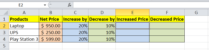
Example: Suppose we buy some products at their net price. We sell these items at an increased rate of 20% on regular days and a reduced rate of 10% from the net prices during the festive season. We need to calculate the increased and decreased prices of products using Excel. In that case, our example Excel sheet would look like this:

To calculate the increased amount by 20%, we use the following formula in cell E2:

=B2*(1+C2)

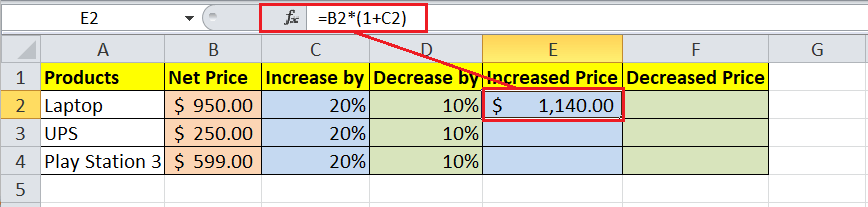
After that, we must drag the formula in other cells, E3 and E4, to calculate the respective increased prices.

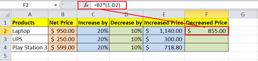
To calculate the decreased amount by 10%, we use the following formula in cell F2:

=B2*(1-D2)

After that, we must drag the formula in other cells, F3 and F4, to calculate the respective decreased prices.

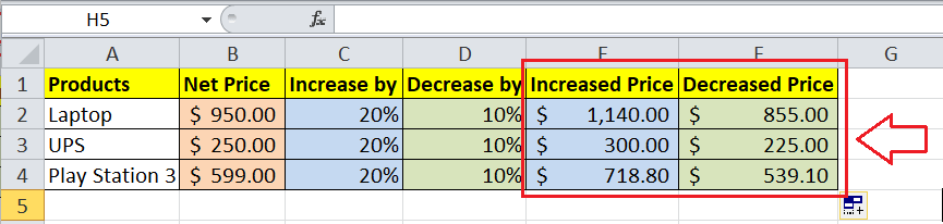
Sellers mainly use this specific case to increase or decrease the price of certain items by a specific percentage in holiday or festive seasons.

Important Points to Remember

• We calculating percentage in Excel, we must ensure that the corresponding cell(s) is formatted in the form of percentage only.
• When dividing the numerator by the denominator, we must ensure that the denominator consists of only non-zero values. If the denominator or a cell used as a denominator contains zero, Excel displays #DIV/0! Error in a result cell.
• The percentage errors are usually removed using Excel’s IFERROR function.