

How To Consolidate Tables With Power Query
I have a worksheet. There are a few tables in there and I’d like to combine them into one table. Power Query will help me with that.
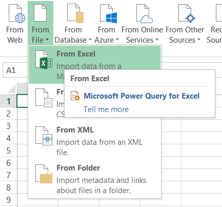
To join tables click Power Query in the ribbon menu. Choose From File – From Excel.
Choose the file in your local drive.
![]()
![]()
Power Query Navigator window pops out.
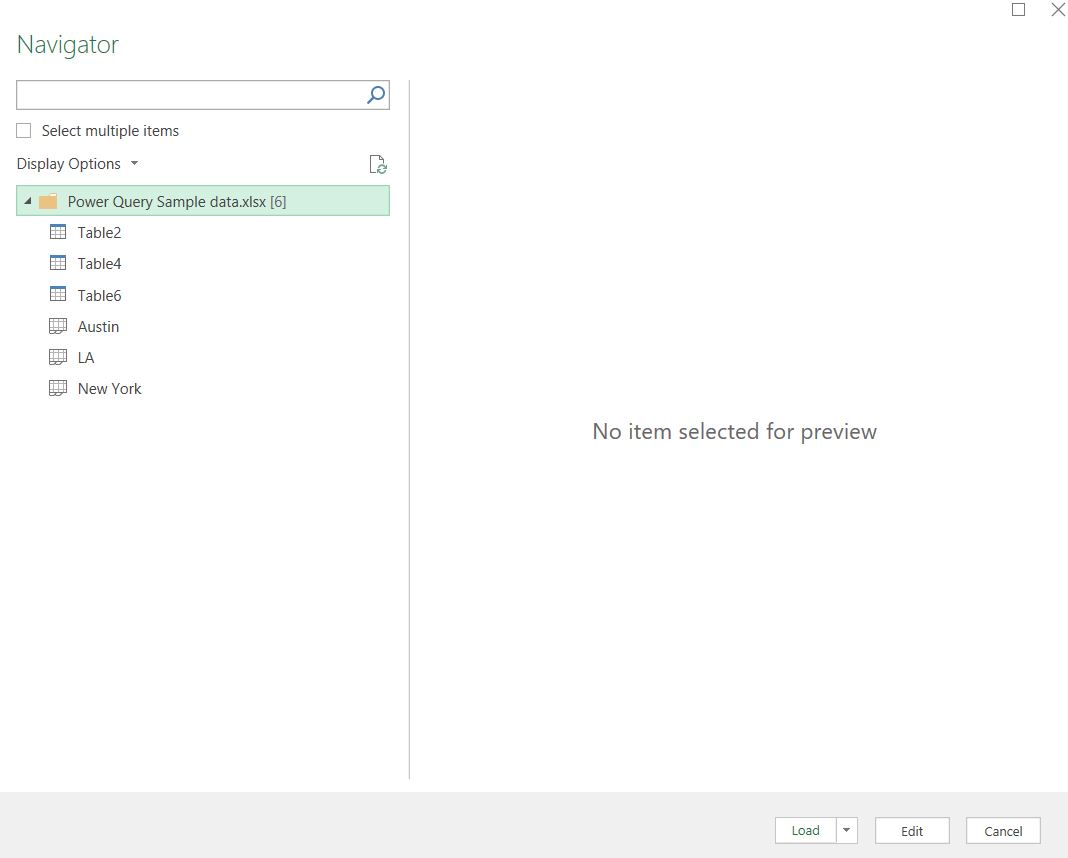
Select the whole file and click Edit.
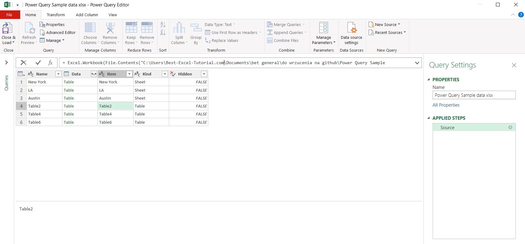
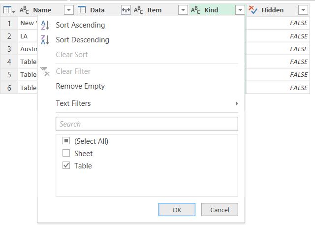
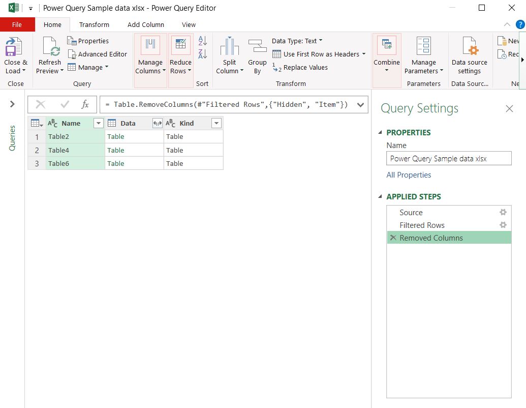
I can see every objects in the whole workbook. I’d like to load only tables. So I need to click Kind and filter only tables.
Next I’d like to remove obsolete columns. I don’t need so many of them.
To merge tables I need to press a small icon next to Data header.
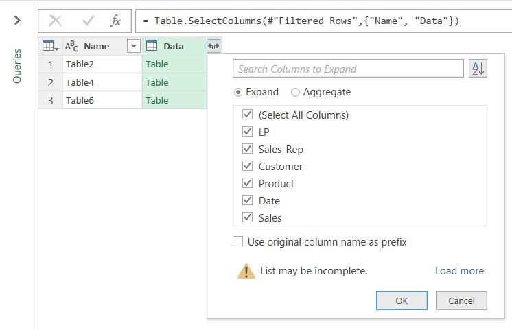
I unchecked Use original column name as prefix option. Just because I don’t like it.
This is how preview of my consolidated tables looks like.
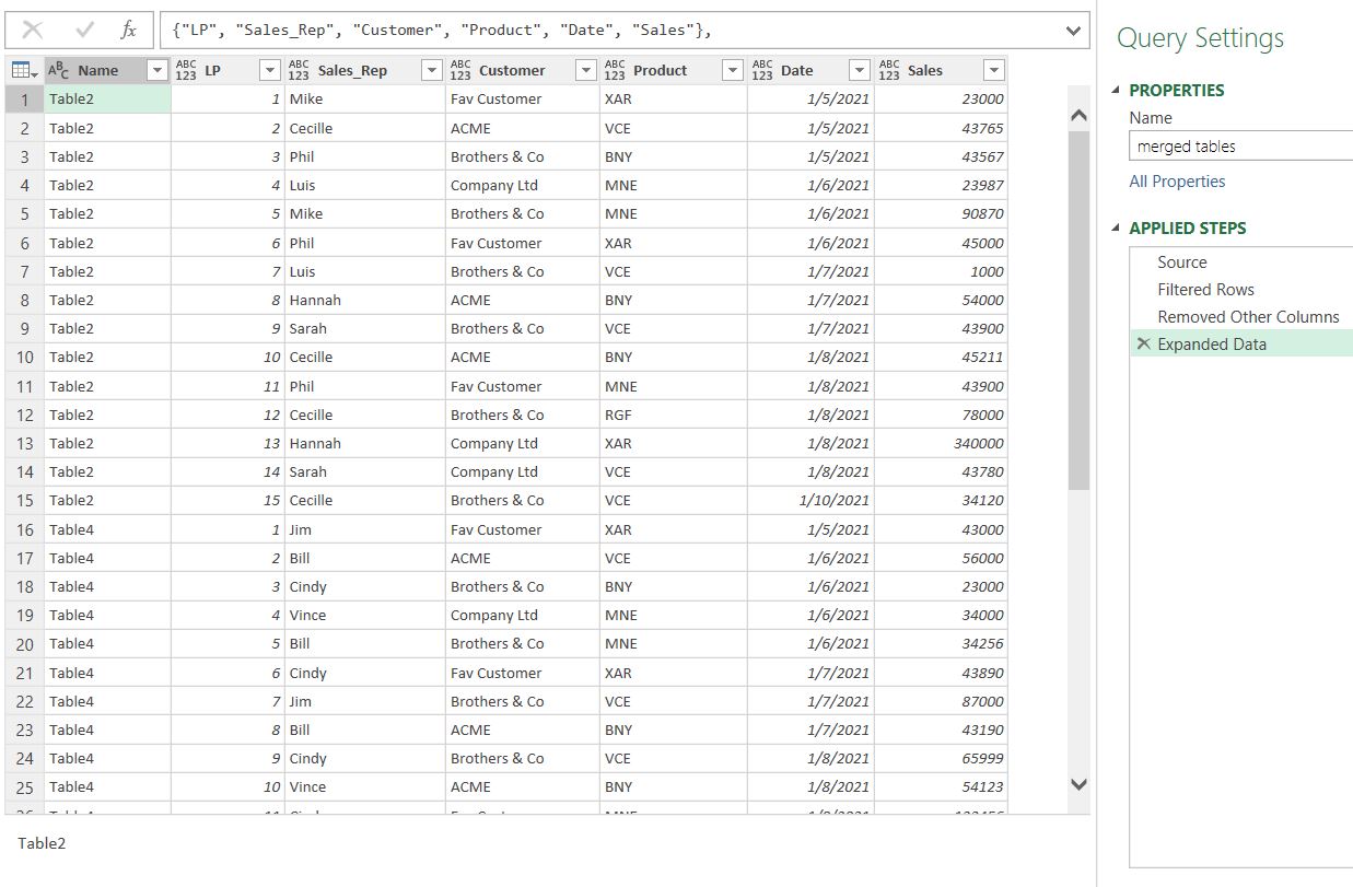
Here is the time for final formatting.
First thing is to change the name. I did it on the right side of the screen.
Next important thing is to set proper columns data formatting. Click the small icon in the top headers and set right data type for each column.
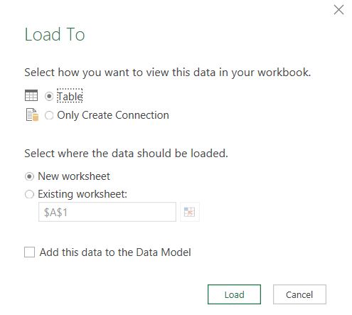
When you are happy from your merged tables, and I am happy, click Close & Load To in the left top side of the screen.
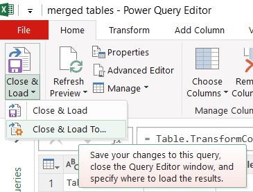
I’d like to have Table in the New worksheet. Click Load to get merged tables in the new sheet.
And here is how my joined tables by Power Query look like.
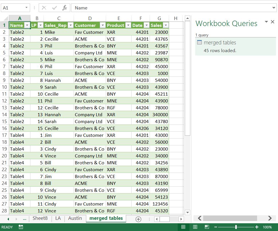
I saved a bunch of time because now I have joined tables which don’t require any more formatting.
Template
Further reading:
Basic concepts
Getting started with Excel
Cell References


