How to Make a Table in Excel?

A table is a powerful feature to group your data in Excel. You can consider a table as a specific set of rows and columns in a spreadsheet. You can have multiple tables on the same sheet. Tables allow you to analyze your data quickly and easily in Excel.

You might think that your data in an Excel spreadsheet is already in a table simply because it’s in rows and columns. However, your data is not in a true “table” unless you used the specific Excel data table feature. You can convert your flat data into a data table with several benefits. Here are some advantages of an Excel table, such as:

• Quick Styles: Add color, banded rows, and header styles with just one click to style your data.
• Table Names: Give a table a name to make it easier to reference in other formulas.
• Cleaner Formulas: Excel Formulas are much easier to read and write when working in tables.
• Auto Expand: Excel tables are dynamic by nature, which means add a new row or column to your data easily, and the Excel table automatically updates to include the new cells.
• Filters & Subtotals: Automatically add filter buttons and subtotals that adapt as you filter your data, such as integrated sort and filter options or visual filtering with slicers.
• Column headings remain visible while scrolling.
• Quick totals allow you to sum and count data and find an average, min, or max values in a click.
• There are easy-to-read formulas due to a special syntax that uses table and column names rather than cell references.
• Dynamic charts adjust automatically as you add or remove data in a table.

How to create a table in Excel

The individual sheets or pages of an Excel spreadsheet resemble tables with their grids of columns and rows. With just a few clicks, you can enter data or import entire datasets into Excel spreadsheets. You can also organize your data into tables without special formatting.

With the source data organized in rows and columns, follow the below steps to covert a range of cells into a table:

Step 1: Select any cell within your data set.

Step 2: Go on the Insert tab and click on the Table button in the Tables group.

Or you can press the Ctrl + T shortcut key to insert a table.

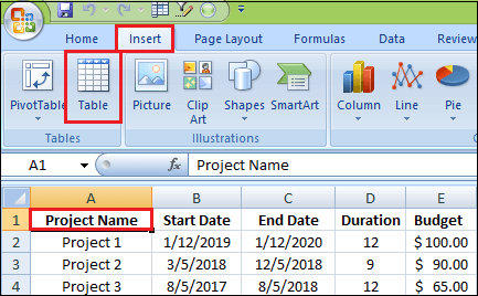
Step 3: The Create Table dialog box appears with all the data selected for you automatically. You can adjust the range and if you want the first row of data to become the table headers, make sure the My table has headers box is selected.

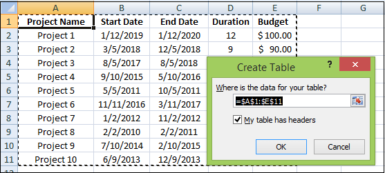
Step 4: Now click on the OK button.

As a result, Excel converts your range of data into a true table with the default style.

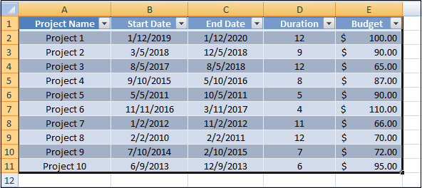
Here are some essential points which need to remember when you create a table in excel.

• Prepare and clean your data before creating a table, remove all blank rows, give each column a unique name, and make sure each row contains information about one record.
• When a table is inserted, Excel retains all formatting that you currently have. For best results, you may want to remove some of the existing formatting, e.g., background colors, so it does not conflict with a table style.
• You are not limited to just one table per sheet. You can have as many as needed. It stands to reason to insert at least one blank row and one blank column between a table and other data for better readability.

How to Name a Table in Excel

Every time you make a table in Excel, it automatically gets a default name such as Table1, Table2, etc. When you deal with multiple tables, changing the default names to something more meaningful and descriptive can make your work a lot easier. To rename a table or give a new name to the table, follow the following steps:

Step 1: Select any cell in the table.

Step 2: Go on the Table Design tab and select the existing name in the Table Name box.

To view all tables’ names in the current workbook, press Ctrl + F3 to open the Name Manager.

Excel Table Formulas

For calculating the table data, Excel uses a special formula syntax called structured references. Compared to regular formulas, they have several advantages, such as:

• Easy-to-create: Select the table’s data when making formula, and Excel will build a structured reference for you automatically.
• Easy-to-read: Structured references refer to the table parts by name, which makes formulas easier to understand.
• Auto-filled: To perform the same calculation in each row, enter a formula in any single cell, and it will immediately be copied throughout the column.
• Changed automatically: When you modify a formula anywhere in a column, the other formulas in the same column will change accordingly.
• Updated automatically: Every time the table is resized or the columns are renamed, structured references update dynamically.

The below image shows an example of a structured reference that sums data in each row:

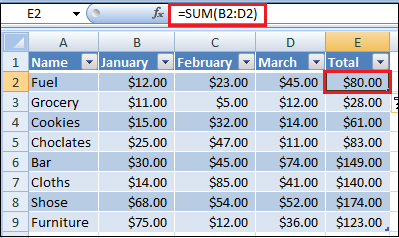
Sum Table Columns

Another great feature of an Excel table is the ability to summarize data without formulas. This option is called Total Row. Follow the following steps to sum a table’s data.

Step 1: Select any cell in the table.

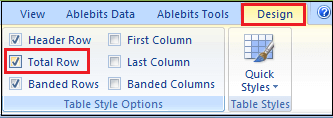
Step 2: Go on the Design tab and put a tick mark in the Total Row box in the Table Style Options group.

Step 3: The Total row is inserted at the bottom of the table and shows the total in the last column.

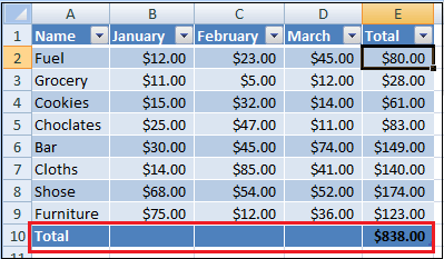
Step 4: Click in the Total cell to sum data in other columns.

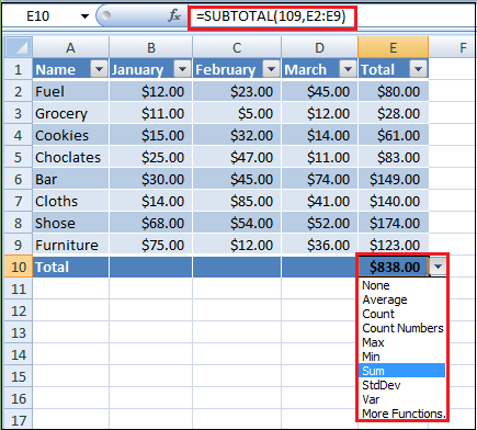
Step 5: Then click the drop-down arrow and choose the SUM function. To calculate data differently, e.g., count or average, select the corresponding function.

Whatever operation you choose, Excel would use the SUBTOTAL function that calculates data only in visible rows.

You can use the Ctrl + Shift + T shortcut key to toggle the Total Row on and off.

How to Extend a Table in Excel

When you type anything in an adjacent cell, an Excel table expands automatically to include the new data. Combined with structured references, this creates a dynamic range for your formulas without any effort from your side.

If you don’t mean the new data to be part of the table, press Ctrl + Z. This will undo the table expansion and keep the data you typed.

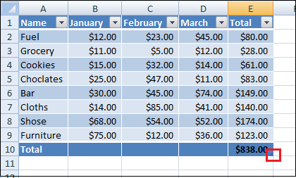
You can also extend a table manually by dragging a little handle at the bottom-right corner.

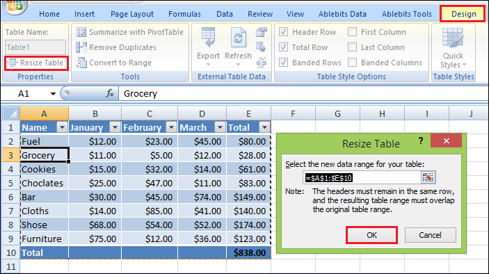
You can also add and remove columns and rows using the Resize Table command with the following steps.

Step 1: Click anywhere in your table.

Step 2: Go on the Design tab and click on the Resize Table in the Properties group.

Step 3: When the dialog box appears, select the range to be included in the table.

Step 4: Click on the OK button.

Excel Table Styles

Tables are very easily formatted due to a predefined gallery of styles. Additionally, you can create a custom style with your own formatting.

When you insert a table in Excel, the default style is automatically applied to it. To change a table style, follow the following steps:

Step 1: Select any cell in the table.

Step 2: Go on the Design tab and click on the style you want to apply from the Table Styles group.

Step 3: To see all the styles, click on the More button in the down-right corner.

NOTE: If you haven’t defined titles for your table columns, Excel automatically adds header placeholders to the table during formatting.

To change the default table style, right-click the desired style and choose Set as Default. Any new table that you create in the same workbook will now be formatted with the new default table style.

When you format a table with any predefined style, Excel preserves the formatting you already have.

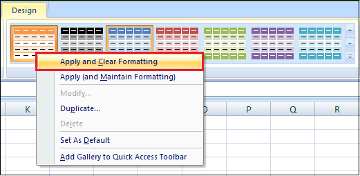
Step 4: To remove any existing formatting, right-click on the style and choose Apply and Clear formatting.

How to Remove Table Formatting

If you would like to have all the functionality of an Excel table but do not want any formatting such as banded rows, table borders, and others, you can remove formatting through these steps, such as:

Step 1: Select any cell within your table.

Step 2: Go on the Design tab and click on the bottom-right corner More button in the Table Styles group.

Step 3: And then click Clear underneath the table style templates. Or pick the first style under Light, which is known as None.

This method only removes the inbuilt table formatting, but your custom formatting is preserved. To remove absolutely all formatting in a table, follow the following way:

Step 1: Go to the Home tab, select the Formats group, and click on the Clear formats button.

NOTE: Unlike custom table styles, predefined styles for Excel tables cannot be deleted. However, you have the option of clearing both predefined and custom styles. The formatting is then removed, and the data is displayed in the default table format.

How to Remove Table in Excel

Removing a table is an easy process. To convert a table back to a range, just follow these steps:

Step 1: Right-click on any cell in your table.

Step 2: Go to the Table button.

Step 3: And then click on the Convert to Range button.

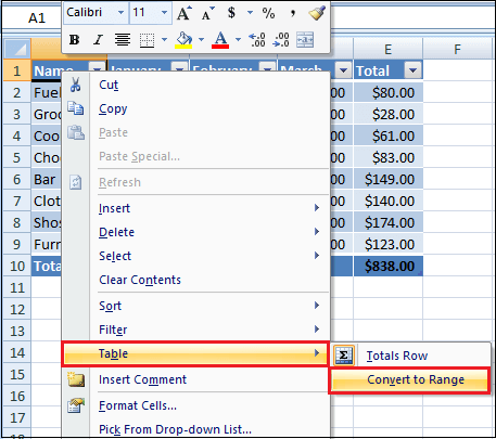
Or go to the Design tab and click on the Convert to Range button in the Tools group.

Step 4: A dialog box appears on the screen, then click on the yes button.

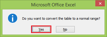
This will remove the table but retain all the data and formatting. To keep only the data, remove table formatting before converting your table to a range.

Drawbacks of Using Excel Table

There are some drawbacks to using named Excel tables, so there might be situations where you prefer not to use them, such as:

• Structured references to table cells don’t have an “absolute” setting, so it’s a bit trickier to copy them across a column.
• Tables won’t expand automatically on protected sheets, even if the cells below the table are unlocked.
• You can’t group and copy or move multiple sheets if any sheet contains an Excel table.
• Custom Views are not allowed in a workbook that has one or more Excel tables.