Hyperlink in Excel

Microsoft Excel, or MS Excel, is one of the most powerful spreadsheet software. It is widely used on different platforms for various purposes. Additionally, it has several excellent features that help users to perform their tasks more efficiently. It provides a wide range of features, allowing users to increase the overall work process’s productivity. One such feature in Excel is a hyperlink, which enables users to link to different internal and external sources. A hyperlink in Excel is such a helpful feature that we should know to work effectively in Excel.

In this article, we are discussing the fundamental concepts of hyperlinks in MS Excel. Additionally, we will also understand how we can insert, remove, or edit hyperlinks to a new file or an existing Excel file. But, first, let’s discuss the definition of the hyperlink and some advantages of using it in Excel:

What is Hyperlink in Excel?

In particular, the hyperlink is used to navigate to a specific web page for most programs. However, Excel provides many more options to perform using a hyperlink. Excel’s hyperlinks are way smarter than as given in other programs. Although we can use a hyperlink in Excel to navigate to any particular web address, we can also use it to navigate to any specific place (cell) within the existing file, open a new file or go to another Excel file.

By definition, “A hyperlink in excel is defined as a reference to any particular location, webpage or a document that we can access or jump to by clicking the link.“

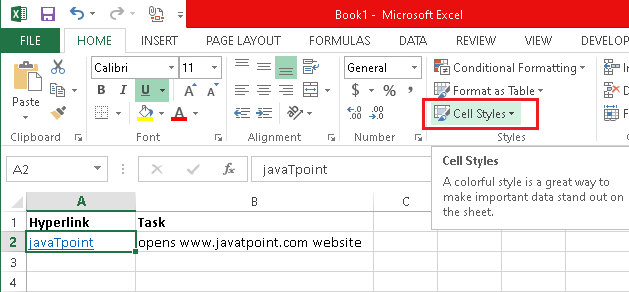
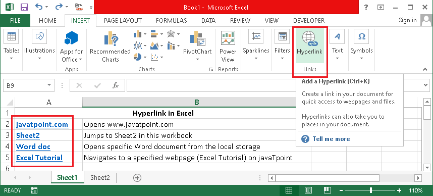
Hyperlinks in MS Excel can be identified easily. Generally, they are the underlined text highlighted in blue color, as shown in the following image:

Apart from the text in a cell, various spreadsheet objects (i.e., images, charts, text boxes, shapes, etc.) can also be combined with clickable hyperlinks.

MS Excel provides support for two types of links, such as absolute and relative. This mainly specifies whether we have used the full address or partial address for creating hyperlinks.

Absolute Hyperlink in Excel

An absolute hyperlink in excel includes a complete address. It contains a protocol and domain name for a used URL, including the full path and the document’s file name. The following are the examples of absolute URLs pointing to internal and external sources:

Example of Absolute URL: (External Source)

https://www.tutoraspire.com/tutorial/excel-tutorial

Example of Absolute Hyperlink: (Internal Source)

C:tutoraspireExcel filesMonthly DataJanuary.xlsx

Relative Hyperlink in Excel

A relative hyperlink in excel includes a partial address without protocol and domain name for URLs. The following are the examples of relative URLs pointing to internal and external sources:

Example of Relative URL: (External Source)

/tutorial/excel-tutorial

Example of Relative Hyperlink: (Internal Source)

Monthly DataJanuary.xlsx

Note: It is strictly recommended to use the full address of URLs (or websites/ webpages) when using hyperlinks in excel. Although Excel can understand URLs without a protocol, it cannot determine a domain name and URLs file path. Besides, we use absolute or relative addresses when creating hyperlinks for excel files or other documents stored on the computer.

Advantages of Hyperlink in Excel

Following are some of the reasons or advantages of using hyperlinks in MS Excel:

• Going to a specific location within the existing workbook
• Opening a current document from the storage or accessing any particular place in any document (i.e., accessing a worksheet in an excel or bookmark in a Word file)
• Navigating to a specific web address on the Internet or Intranet
• Creating a new Spreadsheet (an Excel file)
• Sending an e-mail directly from Excel to a particular e-mail address/ person/ recipient

Types of Hyperlink in Excel

There are mainly six different types of hyperlinks that we can insert in Excel:

• Link from any particular cell to another within the same worksheet
• Link from one worksheet to another within the same spreadsheet file (Excel file)
• Link to a separate file on the computer
• Link to any specific website
• Link to create an E-mail
• Link to create a new file

Let us discuss each type of hyperlink and the process to insert them in Excel:

Link from any particular cell to another within the same worksheet

We can create a hyperlink in any specific cell and link it to another cell in the existing document using the steps given below:

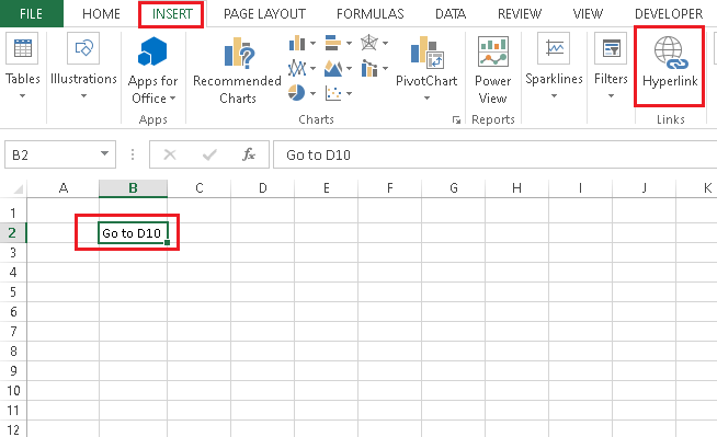
• First, we need to select the cell to insert a hyperlink linking to another cell. Suppose we want to join B2 to D10. This means that every time we click on B2, we will jump from B2 to D10.
• After selecting cell B2, we need to navigate the ‘Insert‘ tab from the toolbar and select the option ‘hyperlink‘.
  
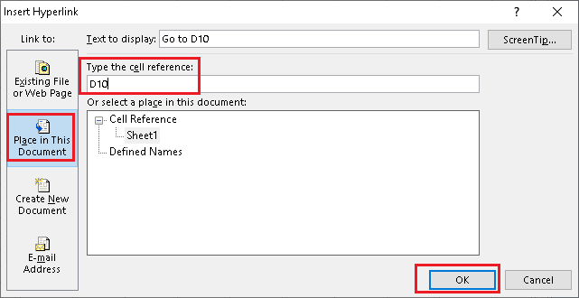
• Next, we need to click on the ‘Place in This Document‘ and enter the text that we want to display on B2 for the hyperlink. Additionally, we must enter the cell reference where we want to jump via a hyperlink created on B2. In our case, it is D10. After putting D10 in the box next to ‘Type the cell reference‘, we need to click on the ‘OK‘ button to save the applied changes.
  
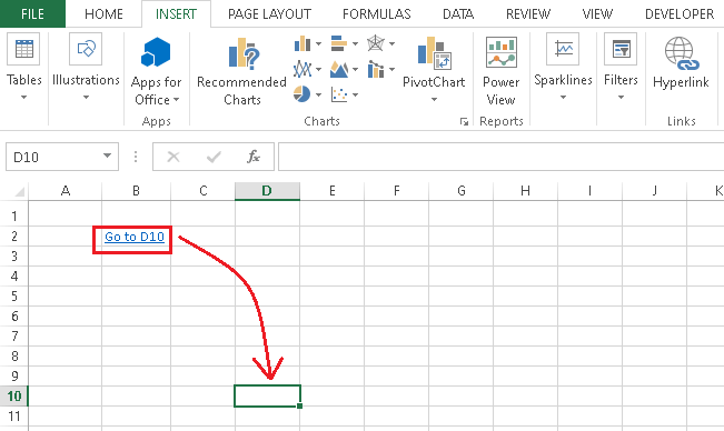
• A cell B2 will turn into a hyperlink (blue and underlined text), and we can click on the hyperlink to jump from B2 to D10.
  

Link from one worksheet to another within the same spreadsheet file (Excel file)

We can create a hyperlink in any specific cell and link it to another worksheet (also called sheets) in the existing document using the steps given below:

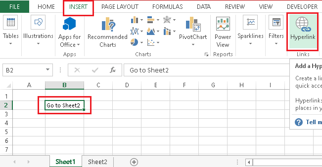
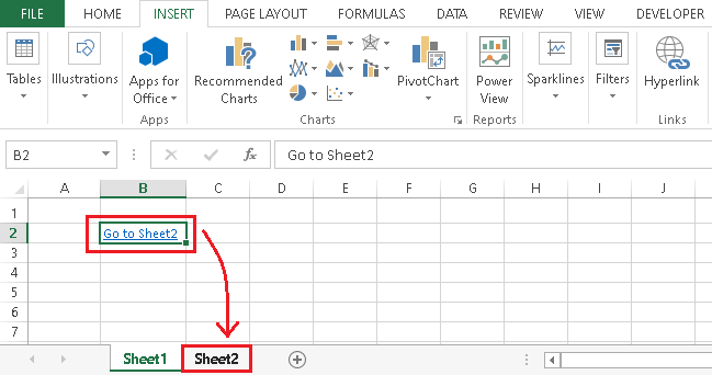
• First, we need to select the cell to insert a hyperlink linking to another worksheet. Suppose we want to connect the B2 cell from worksheet 1 to worksheet 2. This means that every time we click on the B2 cell, we will jump from the B2 cell to worksheet 2 directly.
• After selecting cell B2, we need to navigate the ‘Insert‘ tab from the toolbar and select the option ‘hyperlink‘.
  
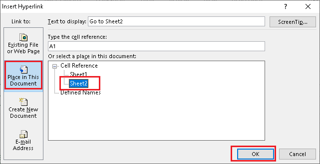
• Next, we need to click on the ‘Place in This Document option and enter the text that we want to display on the B2 cell for a hyperlink. Additionally, we are required to select the particular worksheet where we want to jump via a hyperlink created on B2. In our case, it is Sheet2. After choosing Sheet2 from the ‘Cell Reference’ list, we need to click on the ‘OK‘ button to save the applied changes.
  
  Besides, if we want to jump to any specific cell in Sheet2, then we can enter the particular cell in a box next to ‘Type the cell reference’. By default, it is always A1.
• Finally, a cell B2 will turn into a hyperlink, and we can click on the hyperlink to jump from the B2 cell to worksheet2.
  

Link to a separate file on the computer

We can create a hyperlink in the current excel file to open another file from the local storage. We can link to different excel files, Work files, etc.

To do this, we need to follow the following steps:

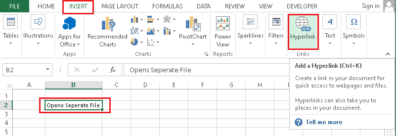
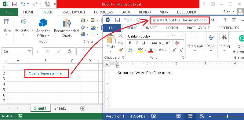
• First, we need to select the cell to insert a hyperlink linking to another file. Suppose we want to connect the B2 cell to a Word file. This means that every time we click on the B2 cell, it will directly launch the associated Word file.
• After selecting cell B2, we need to navigate the ‘Insert‘ tab from the toolbar and select the option ‘hyperlink‘.
  
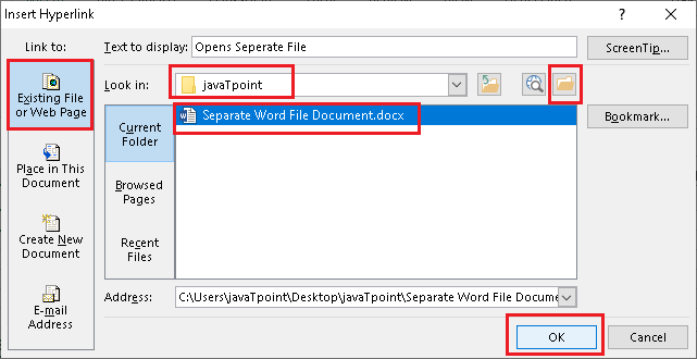
• On the next window, we need to click on the ‘Existing File or Web Page‘ and enter the text that we want to display on B2 for the hyperlink. Additionally, we are required to select the particular file that we want to link via a hyperlink created on B2. In our case, it is Word File named ‘Separate Word File Document’. After selecting the Word file using the file explorer or drop-down list, we need to click on the ‘OK‘ button to save the applied changes.
  
• After that, a cell B2 will turn into a hyperlink, and we can click on the hyperlink to jump from the B2 cell to another Word file, i.e., Separate Word File Document.docx.
  

Link to any specific website

We can also create a hyperlink to launch any specific website directly from an excel cell. To perform this operation, we need to follow the steps given below:

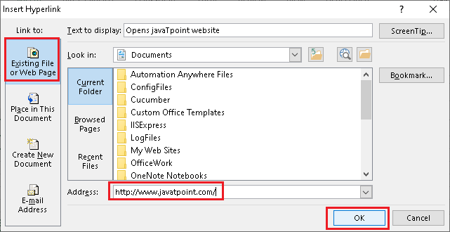
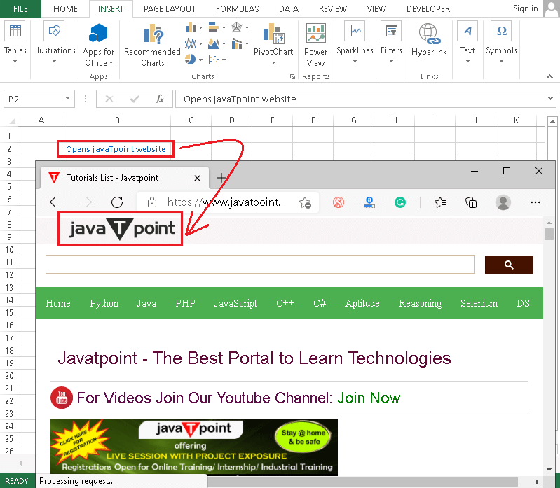
• First, we need to select the cell to insert a hyperlink linking to an external website. Suppose we want to link B2 cell to a website address ‘www.tutoraspire.com’. Every time we click on the B2 cell, it will directly launch the associated website (tutoraspire).
• After selecting cell B2, we need to navigate the ‘Insert‘ tab from the toolbar and select the option ‘hyperlink‘.
  
• On the next window, we need to click on the ‘Existing File or Web Page‘ and enter the text that we want to display on B2 for the hyperlink. Additionally, we must enter the particular website’s URL in a box next to ‘Address’. This will link URL via hyperlink created on B2. In our case, it is the URL of our website. After entering the URL in an address box, we need to click on the ‘OK‘ button to save the applied changes.
  
• After that, a cell B2 will turn into a hyperlink, and we can click on the hyperlink to jump from the B2 cell to a specific website, i.e. ‘www.tutoraspire.com’.
  

Apart from this, we can directly type the web address in a specific cell and press the ‘Enter’ button to create a hyperlink to a website quickly.

Link to create an E-mail

Excel also allows us to use hyperlinks to create and send e-mail to specific user/s automatically. However, it requires Microsoft Outlook or Windows Live Mail software installed on the computer and set as a default application for e-mail. Once configured properly, clicking on a hyperlink in Excel can launch an e-mail application and compose an e-mail with a recipient address.

This can be configured using the steps given below:

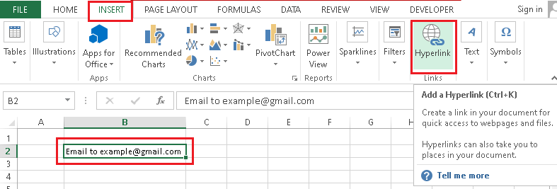
• First, we need to select the cell to insert a hyperlink linking to compose a new e-mail. Suppose we want to link B2 cell to an e-mail address ‘[email protected]‘. This means that every time we click on B2 cell, it will directly launch the default e-mail software and compose a new e-mail to a recipient – [email protected]
• After selecting cell B2, we need to navigate the ‘Insert‘ tab from the toolbar and select the option ‘hyperlink‘.
  
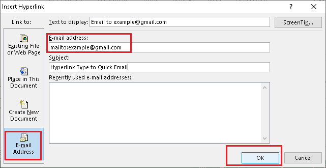
• On the next window, we need to click on the ‘E-mail Address‘ tile and enter the text that we want to display on B2 for the hyperlink. Additionally, we must enter the recipient’s e-mail address in a box next to ‘E-mail address.’ We can then enter the subject if necessary. This will link an e-mail via hyperlink created on B2. Next, we need to click on the ‘OK‘ button to save the applied changes.
  
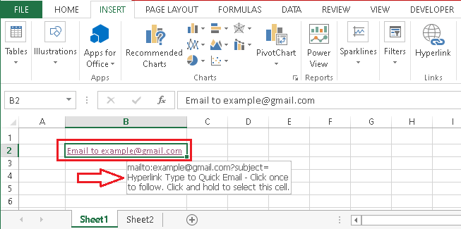
• After that, cell B2 will turn into a hyperlink, and we can click on the hyperlink to create an e-mail with a specified recipient address and a subject.
  

Link to create a new file

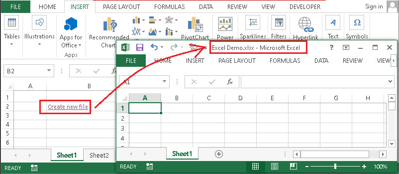
Although this type of hyperlink is not generally used, it can be sometimes beneficial. This type of hyperlink mainly helps to create a new file and edit it instantly with a click. We can insert this hyperlink using the following steps:

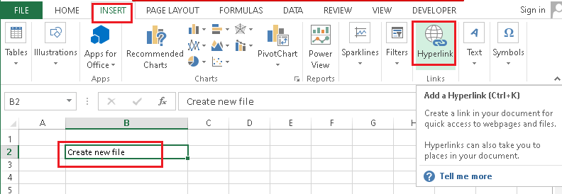
• First, we need to select the cell where we want to insert a hyperlink to create a new document. Suppose we want to link the B2 cell to a new file with the name ‘Excel Demo’. This means that every time we click on the B2 cell, it will directly create a new Excel Demo file. Next, we need to select the specific cell and then go to Insert > Hyperlink.
  
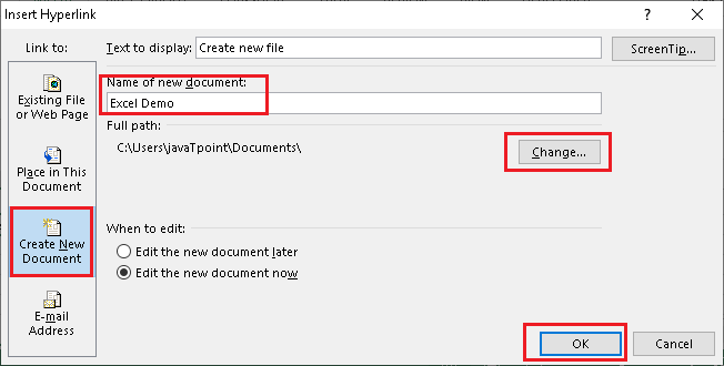
• On the next screen, we need to click on the ‘Create New Document‘ tile. Then, we must enter the name (Excel Demo, in our case) for a new document and select the location to save the file. Additionally, we can choose whether we want to edit the form instantly or later.
  
• Once all the details are filled in, we can click on the ‘OK‘ button, and the particular cell will convert to a hyperlink.
  
  We can click on the hyperlink to create a new file with corresponding details.

Editing an existing Hyperlink

If we have an excel workbook containing more or fewer hyperlinks and a need to modify them, we can efficiently perform this task. However, we should have admin permission to access and modify the particular file.

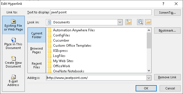
To perform this task, we must first select the specific cell with a hyperlink and then click on the hyperlink tile by navigating to Insert > Hyperlink.

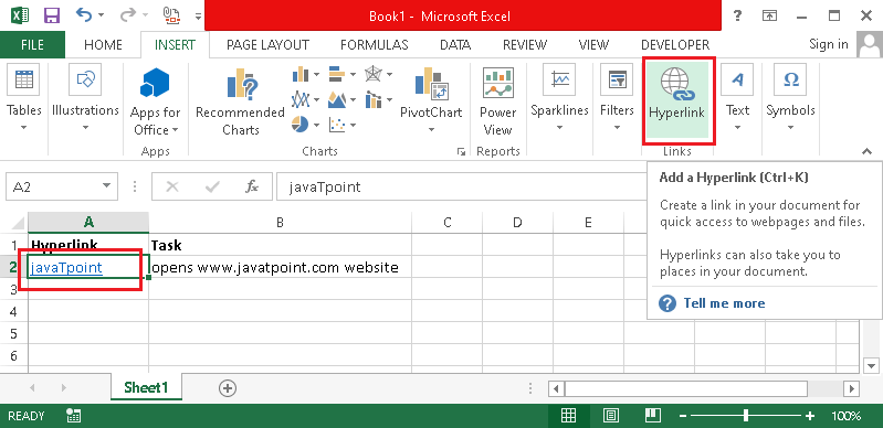
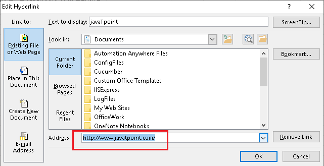
After doing this, a new window (Edit Hyperlink Window, shown in the following image) appears to replace or edit the details or links accordingly.

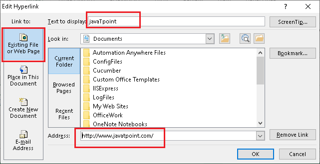
Once we are done modifying the details, we need to click on the ‘OK’ button, and all the details will be updated instantly. It is essential to save the file changes to avoid doing the same modification again and again.

Apart from this, we can also follow another simple method for editing hyperlinks in Excel. According to this method, we must find the cell with a hyperlink that we want to edit. Next, we need to right-click on the cell and click on the ‘Edit Hyperlink‘ button from the menu options. This looks like the following image:

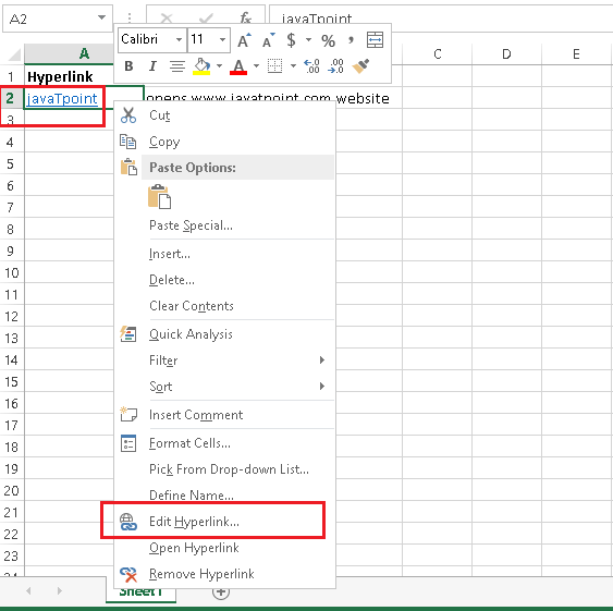
This will also open the same window or edit window, which we can use to make changes to the hyperlink accordingly.

In addition to the editing hyperlinks, we can alternately change the appearance of hyperlinks in our workbook. By default, Excel’s hyperlinks are traditional blue-colored texts with underlines and links (or reference/ place). To edit the default formatting in Excel, we can follow the steps discussed below:

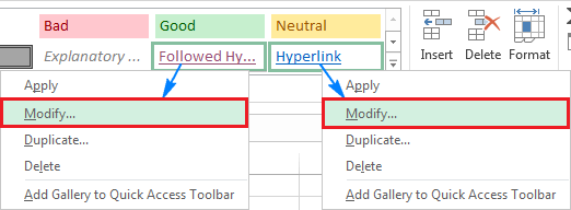
• First, we need to navigate to Home > Cell Styles from the ‘Styles’ section from the toolbar.
  
• Next, we can right-click on the ‘Hyperlink‘ and then click on the ‘Modify‘ option from the menu list. This option is mainly used to change the appearance of the hyperlinks where we have not clicked. Besides, we can right-click on the ‘Followed Hyperlink’ and then click on the ‘modify’ option to further change the hyperlinks’ appearance where we have previously clicked.
  
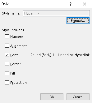
• After clicking on the ‘Modify’ option, a new window will appear, including different styling options. Here, we need to click on the ‘Format‘ button.
  
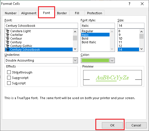
• We can switch to different tabs on the next window (Format Cells) to change the formatting accordingly. For example, we can click on the ‘Font’ tab and apply the various styling such as font, font style, size, color, etc. Once we are done editing the formatting, we need to click on the ‘OK’ button to save the current workbook changes.
  

• In case the applied formatting doesn’t look good, we can follow the entire procedure again to change it to other styles or use ‘Ctrl + Z’ to undo the applied changes and come back to default formatting.

Removing Hyperlink in Excel

Removing or deleting the hyperlinks in Excel is very easy. All we have to do is to follow a two-step process, as discussed below:

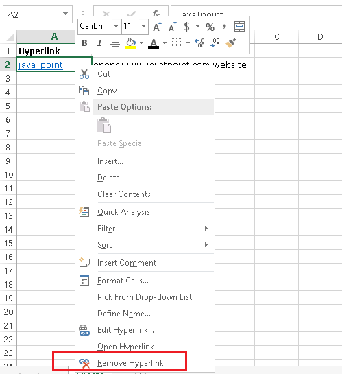
• First, we are required to find a specific cell with a hyperlink that we want to remove. We need to right-click on a particular cell.
• Next, we need to click on the ‘Remove Hyperlink‘ option from the menu list, and the hyperlink will be converted to regular text.
  
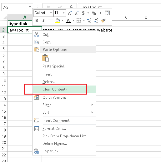
  It is important to note that the method only removes clickable hyperlinks. In case we also want to remove the text, we need to right-click on the cell and click on the ‘Clear Contents’. This will remove the text associated with the hyperlink that we have removed using the previous step.
  

Useful Tips for Hyperlinks in Excel

The following are some useful tips to work with hyperlinks most efficiently in Excel:

Quick Shortcut for Hyperlink Window

Instead of using a hyperlink tile from the toolbar or the right-click options, we can also use a keyboard shortcut to open a window to add/ edit hyperlinks quickly. We have to select a particular cell where we want to add/edit a hyperlink and press ‘Ctrl + K‘ from the keyboard. This will instantly launch the ‘Edit Hyperlink’ dialog and display the corresponding window.

Selecting a Cell containing a Hyperlink

By default, when we try to select the cell containing a hyperlink by clicking on it, it automatically redirects us to the link destination (such as a website, webpage, another document, or cell). To select a cell without navigating to a link target, we are first required to click the cell and keep the mouse button clicked (pressed) until the pointer sign changes to a plus sign (Excel selection cursor). Once the plus sign has arrived, we can release the mouse button, and the specific cell will be selected.

The second method to select a cell is to click on the empty area of the cell. Again, when we move the cursor in an empty area, the cursor sign must be changed into a plus sign. If there is no empty area, we can drag and increase the width of a specific cell.

One more method is to select the cell containing a hyperlink is to select the neighboring cell and then use the arrow keys and reach on a specific link cell.

Extracting Links (URLs) from Hyperlinks

The simplest method to extract a URL from a hyperlink includes the following steps:

• First, we need to select the cell where there is a hyperlink.
• Next, we need to use the shortcut Ctrl + K or go to Insert > Hyperlink.
• On the new window (Edit Hyperlink), we can select and copy the URL from the address input field.