Hypothesis Testing in Excel
Hypothesis t-Test Testing using T.Test Excel function
To test t test hypotesis in Excel you can just use T.Test function. The syntax of T.TEST Excel function:
- Array1: the first set of data to test
- Array2: the second set of data to test
- Tails: the number of tails where 1. is one-tailed distribution and 2 is for two tailed distribution
- Type: 1 is for paired, 2 for homoscedastic, 3 for heteroscedastic
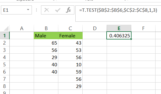
This is the data set and two arrays for my t hypothesis. I’d like to test the hypothesis if the is a difference in given arrays.

The formula I used for T-Test hypothesis is
=T.TEST($B$2:$B$6,$C$2:$C$8,1,3)
because the variance of these arrays is different.

Now we need to interpret the calculated probability. Calculated p ≥ 0.05 means that difference is not significant and p ≤ 0.05 means that difference is significant. The hypothesis result is 0.406325 so the difference is not significant.
Hypothesis T-Test Testing using Analysis Toolpak Add-in
There is also a possibility to perform the same t hypothesis testing using Analysis Toolpak Add-in.
1. Click on Data on the top, beside formula.
2. Click Data analysis.

Note: The data analysis is quite standard. But if it does not show under the data, then it is more likely that it has not been added, which could be done by clicking on File > Options > Add-Ins > Clicking Go on the down side when manage shows Excel Add-ins, and then choosing Data Analysis, and it will be ready.
3. Browse the Data Analysis, and choose the t-text: two-sample assuming unequal variances (1), and press ok (2).

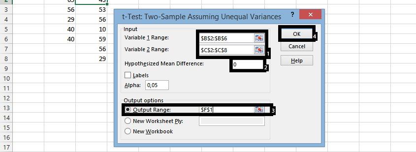
4. Select the data for the two columns (1), write 0 in the Hypothesized mean difference (2), select the cell desired in the output range (3), and press ok (4).

And this is how to handle Hypothesis Testing in Excel.
Template
Further reading:
Basic concepts
Getting started with Excel
Cell References


