

Monte Carlo Simulation In Excel
Let’s say you rule the company. The business is tough so risk of your business is high. You need to be extremely careful.
The task is to check if it is a good idea to introduce a new product to the market.
Perform Monte Carlo simulation to calculate profitability of a new product and calculate probability of profit.
You had a talking with your experts so you know some data:
- fixed costs $80,000-$110,000 depends on resources costs
- number of clients 400-500
- unit price $215
To perform Monte Carlo simulation of introducing a new product to the market in Excel first you need spreadsheet with data.
Columns are:
- lp – just for a reference – let’s prepare 10,000 simulations – the more the better
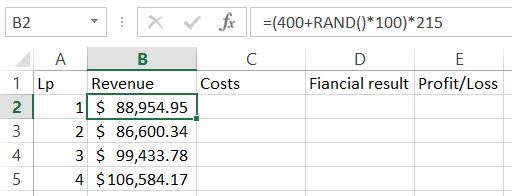
- revenue – number of clients multiplied by unit price to calculate how much money the new product will earn
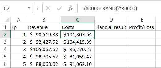
- costs – 80,000 – 110,000 as we got the info from our resources department
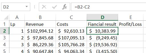
- financial result to check what is the difference between revenue and costs – this we will need to calculate average profit
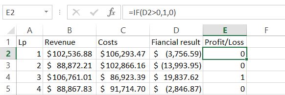
- profit/loss to see if the financial result is above zero – this we will need to calculate probability of profit
Monte Carlo simulation is all about random numbers. We don’t know costs and clients so we need to generate random numbers in Excel to perform the simulation. Luckily there is RAND function in Excel which will generate random numbers for us.
To understand the base of simulation you need to understand how Excel RAND function works:
- RAND function is randomly generating the number between 0 and 1.
- to get the number between 0 and 100 you need just to multiply the result of RAND function by 100. The formula will be =RAND()*100
- to simulate 200 – 300 range just add 200 for that using formula =RAND()*100+200
I hope you understand that. Better read these points a few times to fully understand the clue of that to fully understand Monte Carlo simulation.
You can use RANDBETWEEN Excel function if you don't care
about forecast accuracy so much.
It will generate integers in given range when
RAND is generating decimals.
Let’s move on with calculations.
To calculate revenue I used
=(400+RAND()*100)*215 formula:
- remember that number of clients is 400-500
- 400+RAND()*100 will generate random number between 400 – 500
- unit price is 215 and I need to multiply random number of clients in range between 400 and 500 to get total sales
Apply formula to entire column.
Next one is cost. Similarly formula is
=(80000+RAND()*30000) to generate random number in range 80,000 – 110,000.
To calculate financial results you just need to know how to subtract in Excel.
The formula is =B2-C2.
For the next Profit/Loss column we need to know if it is true or not. Let’s agree that for profit we will see 1 and 0 will be for loss. IF Excel function will do the job!
The formula is
=IF(D2>0,1,0)
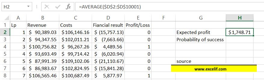
Now we are able to calculate average of expected profit. Of course there is dedicated function for that. Average Excel function will calculate it.
The formula is
=AVERAGE($D$2:$D$10001)
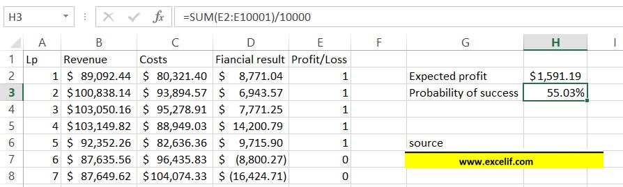
To calculate probability it is enough to sum column E.
Excel Sum function will do the job.
The formula is
=SUM($E$2:$E$10001)/10000
Hit F9 keyboard key several times. Please notice that the numbers change slightly. The more rows the smaller the changes will be.
Monte Carlo simulation is finished. Now based on the number you can decide if it is worth to take the risk and introduce the product into the market.
Excel did the job, now it is on you to take a call.
Template
Further reading:
Basic concepts
Getting started with Excel
Cell References


