Excel Pivot Chart: Dynamic Data Visualization

Pivot Chart in Excel

Pivot Chart is similar to the traditional, but has some additional features useful for the analysis of data.

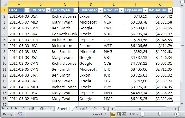
I have prepared table with sales data:

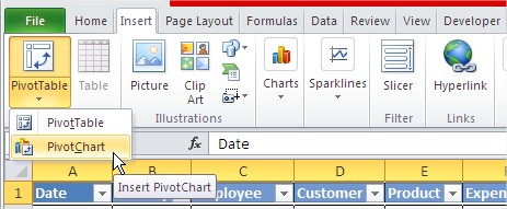
Next go to Ribbon. Click Insert -> Pivot Table -> Pivot Chart

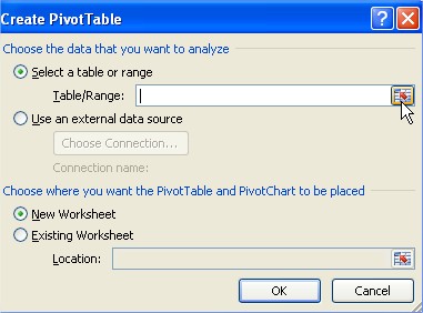
Dialog box appears. Choose here range of table with headers.

Now you can create your own Pivot Chart.

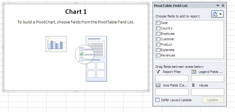
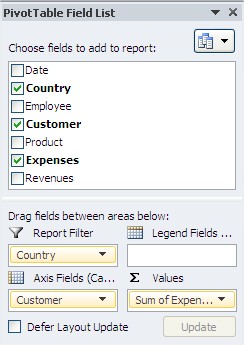
Choose fields which you want to put on the Pivot Chart.

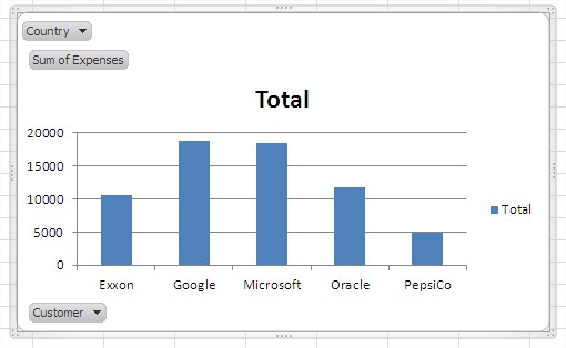
Here’s how the Pivot Chart looks. In fact it is a better version of Column Chart.

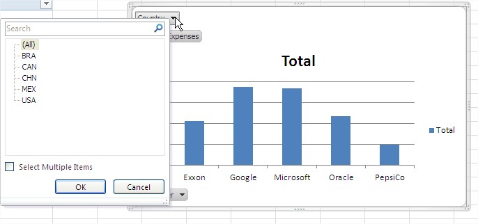
You can click Country or Customer button to filter values.

Excel inserted also a Pivot Table in your Spreadsheet.

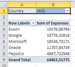
You can change Pivot Chart by changing this Pivot Table. Pivot Chart shows the same values which you see in this Pivot Table.

Try to update / filter / change data in Pivot Table and see, how the Pivot Chart changed.

Template

Further reading: 
Basic concepts 
Getting started with Excel
Cell References