How To Insert Two Chart Types In One Chart
Do you know that you can create one chart with two different types? It is really easy!
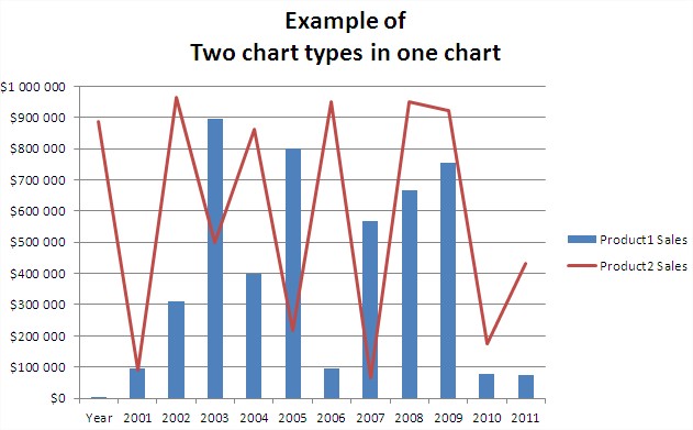
I show you some simple example of two chart types in one chart.
First prepare some data. I have some simple table with sales data about two products.
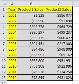
Next go to ribbon, click Insert and choose Column Chart.

Create blank column chart.
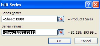
Click right on the chart and choose Select Data option. Now let’s add some Series.
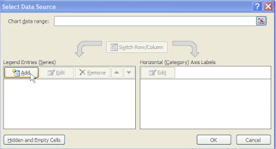
Series name is =Sheet1!$B$1 and Series Values is =Sheet1!$B$2:$B$13
The same way click Edit Category and type Axis Label Range =Sheet1!$A$1:$A$13 and click OK.

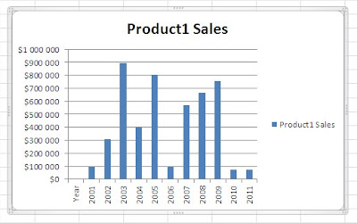
Thats how your chart looks like right now:
To insert Product2 Sales to chart just select Column C in the table…
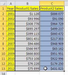
… press Ctrl + C keyboard shortcut to copy, click on the chart and press Ctrl + V to paste the data into the chart. Now you have two columns into your chart.
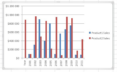
To change the type of the chart, first click on the red column to select all red columns.
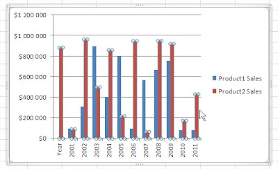
Click right on the one of them and select Change Series Chart Type.
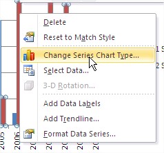
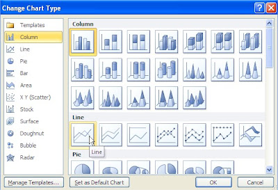
In th dialog box choose Line Chart and accept OK.
Here it is! Now there are two different types of chart! Columns and line in the one chart!
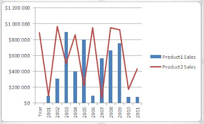
Little more formatting and you have your two charts ready. Isn’t it simple?

Template
Further reading:
Basic concepts
Getting started with Excel
Cell References


