Excel Age Population Pyramid: Demographic Visualization

Pyramid Information Layout

You should layout the data. Don’t bother about the rest at the moment.

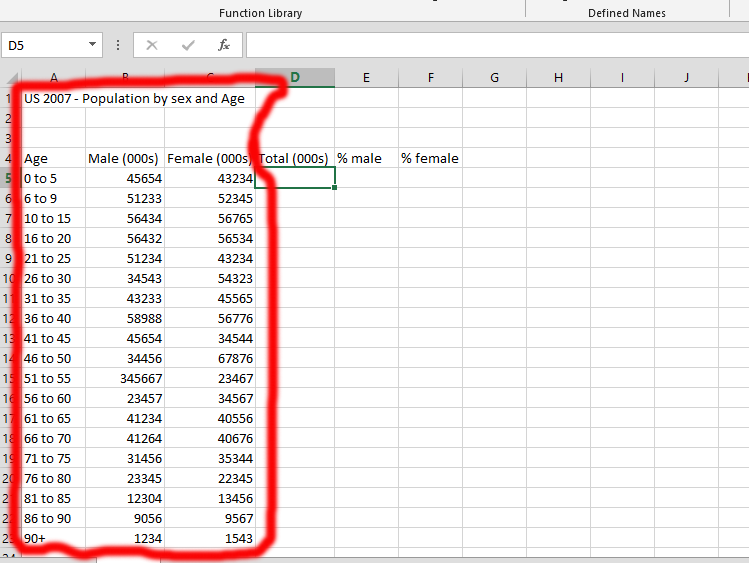
Mark the columns that you are going to calculate. There are female and male, and we are going to do the total calculation of all at the same time. Click on three rows, just as it is marked in the one labeled as number 1. You could find the AutoSum in the “home” tab. You could also go the formulas, which is labeled number 2, and finally press AutoSum, labeled number 3, and just click on it.

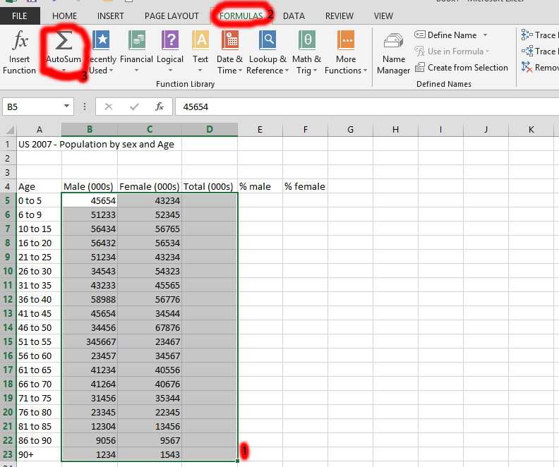
Mathematical Workout

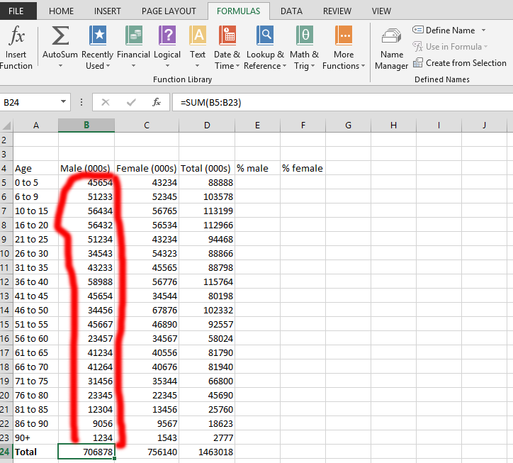
Mark the rows, beginning with the one marked in red, and then click on AutoSum to calculate the total of the rows. Do the same thing with all the rows.

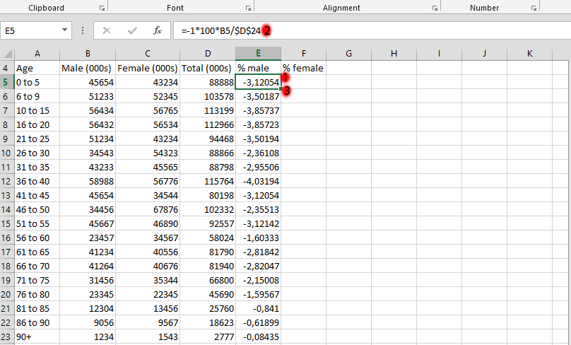
Click on the column, as the one marked as number 1 has made, and then type in the same thing showing in one labeled as number 2. Click on the column beneath the one you have just calculated, and then type in =-1*100*B6/D24. Click on the small square showing beside number 3, the one marked in green, and drag it down to the last column. If that does not work for you, continue doing the number 1, and number 2 on all the columns.

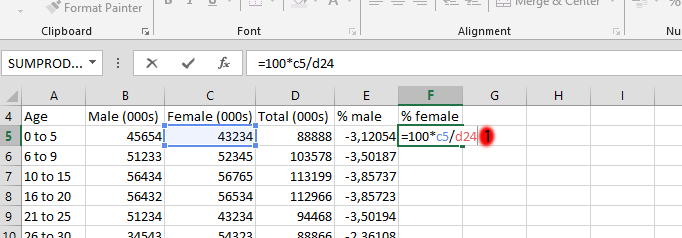
You are going to choose the column where you would like to place the result of the calculation. As it is written in number 1, and then type in the calculation, and choose the column you would calculate, using the sumproduct function in Excel. You should continue doing the same thing in all the columns you would like to calculate using the same thing written in number 1 in the picture above.

Pyramid Chart Creation

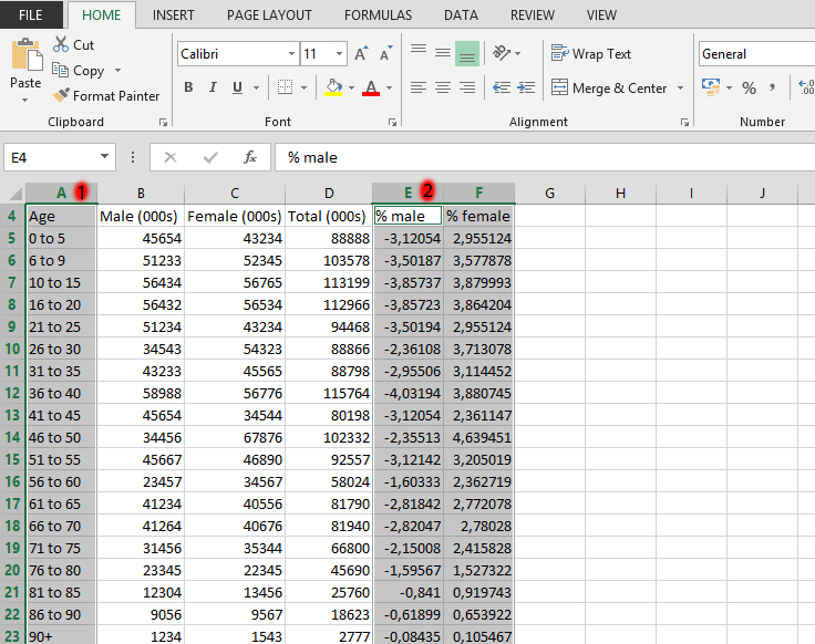
Choose the age row, all the way down, as it is labeled as number 1. Then, you should press CTRL button on your keyboard, while clicking on the area that is marked as number 2, and choose the whole rows, with your keyboard arrows, and SHIFT button. You should not choose the total row though.

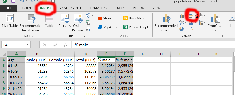
Click on insert tab, as marked in the number 1, and then choose the 2D-Bar chart, as marked in number 2. Then choose the chart.

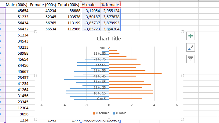
The chart should look like this.

Population Adjustment

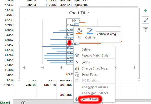
Right click on the axis. The axis has to be marked as you’d see in the number 1 area. Then click format axis, which is marked in red, and labeled number 2.

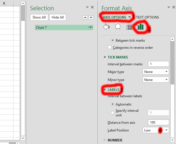
In the format axis, you should choose the axis option (if it is another thing showing). This is the one labeled as number 1. Then you should choose the chart symbol, which is the one labeled number 2. Then click on labels, which is the number 3, and finally choose low in the label position, which is labeled number 4.

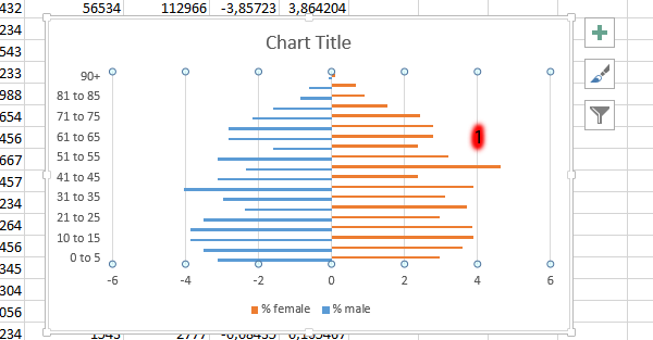
Click on the lines, the one marked number 1. Clicking on it make all the lines showing that they have been marked.

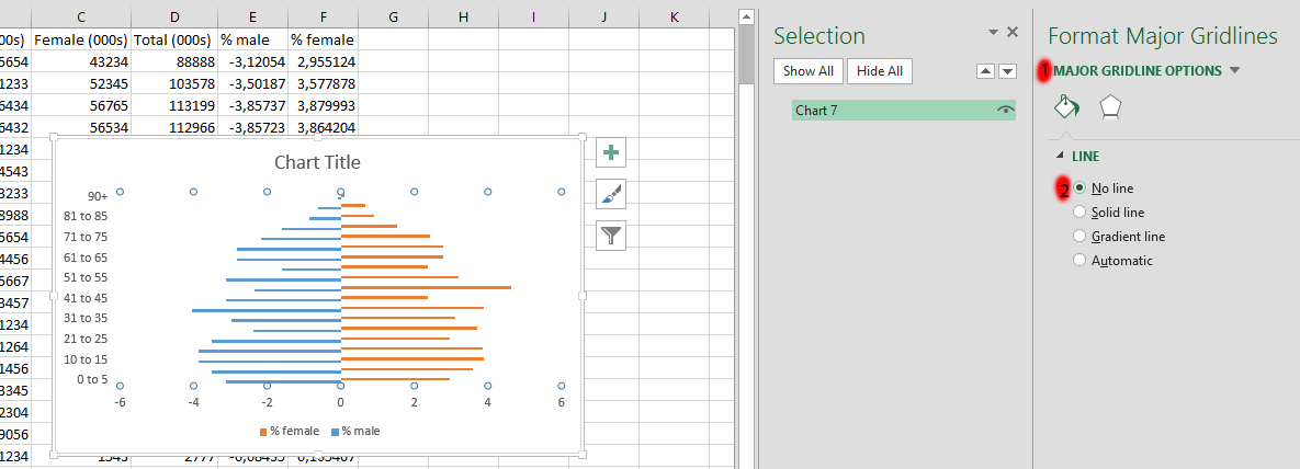
Once you have clicked on the lines, your Microsoft Excel should show the major gridlines option, and if it does not, you should click on it. This is the one labeled as number 1. You should see the line in this options, just click on no line, which is the one labeled number 2.

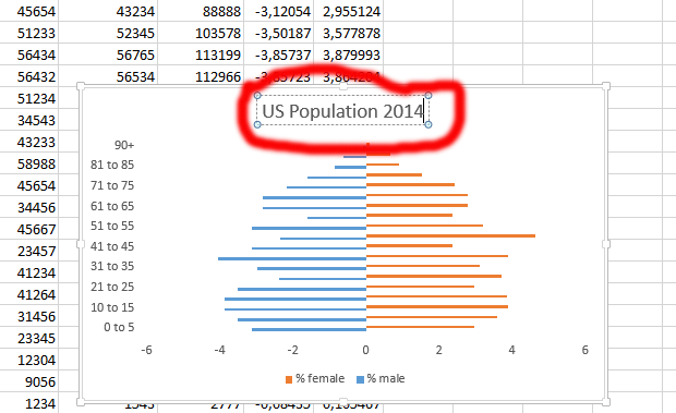
Click on the chart title, and type in the title of your chart.

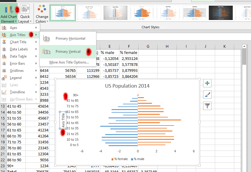
In the one marked as number 1, you should right click with your mouse, this would marked that axis. Then you should click on the number 2, which is “add chart element”, and then choose the “axis title”, marked number 3, and then choose “Primary Vertical”, marked number 4. The one labeled number 5, is the place where you would be writing the axis title.

Designing the Chart

You should click on the chart you have created, and you would be able to see the design tab, and if you do not, click on the design tab, marked in red, labeled number 1, then choose the desired design, which is marked as number 2. Finally, you could also decide to change the colors of the charts, using the one marked as number 3, “change colors”.

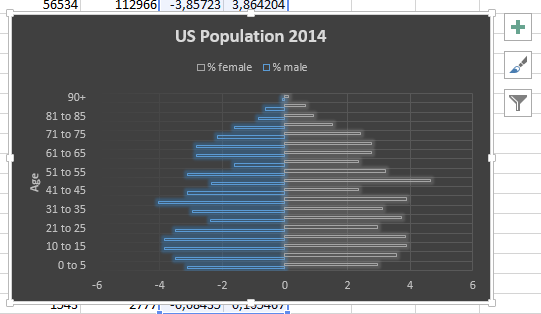
That is how the age population graph would look like when you are done.